Top

Q-learning

• Estimator
• Implementation
• Analysis
• Methods

Q-learning can be viewed as a generalization of the regression-based estimation of a single decision optimal regime discussed previously in Chapter 3. Recall, an optimal regime is represented in terms of Q-functions; namely,

\[ Q_{K}(h_{K},a_{K}) = Q_{K}(\overline{x}_{K},\overline{a}_{K}) = Q_{K}(\overline{x},\overline{a}) = E(Y|\overline{X} = \overline{x}, \overline{A} = \overline{a}), \]

and, for \(k=K-1,\ldots,1\),

\[ Q_{k}(h_{k},a_{k}) = Q_{k}(\overline{x}_{k},\overline{a}_{k}) = E\{ V_{k+1}(\overline{x}_{k},X_{k+1},\overline{a}_{k}) |\overline{X}_{k} = \overline{x}_{k}, \overline{A}_{k} = \overline{a}_{k}\}. \]

Further, for each decision point, \(k = 1, \dots, K\), the value is defined as

\[ V_{k}(h_{k}) = V_{k}(\overline{x}_{k},\overline{a}_{k-1})= \max_{a_{k} \in A_{k}} Q_{k}(h_{k},a_{k}). \]

Q-learning is based on direct modeling and fitting of the Q-functions. In the standard Q-learning approach, one posits parametric models for the Q-functions

\[ Q_{k}(h_{k},a_{k}; \beta_{k}) = Q_{k}(\overline{x}_{k},\overline{a}_{k}; \beta_{k}), \hspace{0.1in} k=K,K-1,\ldots,1. \]

The posited models can be linear or nonlinear in \(\beta_{k}\) and include main effects of and interactions among the elements of \(\overline{x}_{k}\) and \(\overline{a}_{k}\). Given these models for the Q-functions, estimators \(\widehat{\beta}_{k}\) for \(\beta_{k}\) are obtained in a backward iterative fashion for \(k=K,K-1,\ldots,1\) by solving suitable M-estimating equations, such as those corresponding to ordinary or weighted least squares.

A general implementation of the steps of the Q-learning algorithm is provided in R package DynTxRegime through function qLearn(). This function was previously discussed in the context of single decision point analyses in Chapter 3. For multiple decision point analyses, the Q-learning algorithm is accomplished through repeated calls to function qLearn() as we illustrate in the Analysis section.

A general implementation of the Q-learning algorithm is provided in R package DynTxRegime through repeated calls to function qLearn().

R Function

The function call for DynTxRegime::qLearn() can be seen using R’s structure display function utils::str()

utils::str(object = DynTxRegime::qLearn)

function (..., moMain, moCont, data, response, txName, fSet = NULL, iter = 0L, verbose = TRUE)  

We briefly describe the input arguments for DynTxRegime::qLearn() below

Input Argument	Description
\(\dots\)	Ignored; included only to require named inputs.
moMain	A “modelObj” object or a list of “modelObj” objects. The modeling object(s) for the \(\nu_{k}(h_{k}; \phi_{k})\) component of \(Q_{k}(h_{k},a_{k};\beta_{k})\).
moCont	A “modelObj” object or a list of “modelObj” objects. The modeling object(s) for the \(\text{C}_{k}(h_{k}; \psi_{k})\) component of \(Q_{k}(h_{k},a_{k};\beta_{k})\).
data	A “data.frame” object. The covariate history and the treatments received.
response	For Decision K analysis, a “numeric” vector. The outcome of interest, where larger values are better. For analysis of Decision k, k = 1, …, K-1, a “QLearn” object. The value object returned by qLearn() for Decision k+1.
txName	A “character” object. The column header of data corresponding to the \(k^{th}\) stage treatment variable.
fSet	A “function”. A user defined function specifying treatment or model subset structure of Decision \(k\).
iter	An “integer” object. The maximum number of iterations for iterative algorithm.
verbose	A “logical” object. If TRUE progress information is printed to screen.

Value Object

The value object returned by DynTxRegime::qLearn() is an S4 object of class “QLearn”, which stores all pertinent analysis results in slot @analysis.

Slot Name	Description
@step	The step of the \(Q\)-learning algorithm to which this object pertains.
@analysis@outcome	The outcome regression analysis.
@analysis@txInfo	The treatment information.
@analysis@call	The unevaluated function call.
@analysis@optimal	The estimated value, \(Q\)-functions, and optimal treatment for the training data.

There are several methods available for objects of this class that assist with model diagnostics, the exploration of training set results, and the estimation of optimal treatments for future patients. We explore some of these methods under the Methods tab.

• Step 1
• Step 2
• Step 3

The Q-learning algorithm begins with the analysis of Decision \(K\). In our current example, \(K=3\).

moMain, moCont, iter

Inputs moMain and moCont are modeling objects specifying the model posited for \(Q_{3}(h_3, a_3) = E(Y|\overline{X} = \overline{x}, \overline{A} = \overline{a})\). We posit the following model

\[ \begin{align} Q_{3}(h_{3},a_{3};{\beta}_{3}) =& {\beta}_{30} + {\beta}_{31} \text{CD4_0} + a_{1}~({\beta}_{32} + {\beta}_{33} \text{CD4_0}) \\ & + {\beta}_{34} \text{CD4_6} + a_{2}~({\beta}_{35} + {\beta}_{36} \text{CD4_6})\\ & + {\beta}_{37} \text{CD4_12} + a_{3}~({\beta}_{38} + {\beta}_{39} \text{CD4_12}), \end{align} \]

which is defined as a modeling objects as follows

q3Main <- modelObj::buildModelObj(model = ~ CD4_0*A1 + CD4_6*A2 + CD4_12,
                                  solver.method = 'lm',
                                  predict.method = 'predict.lm')

q3Cont <- modelObj::buildModelObj(model = ~ CD4_12,
                                  solver.method = 'lm',
                                  predict.method = 'predict.lm')

Note that the formula in the contrast component q3Cont does not contain the treatment variable; it contains only the covariate(s) that interact with the treatment.

Both components of the outcome regression model are of the same class, and the models should be fit as a single combined object. Thus, the iterative algorithm is not required, and iter=0, its default value.

To see a brief synopsis of the model diagnostics for this model, see header \(Q_{k}(h_{k},a_{k};\beta_{k})\) in the sidebar menu.

data, response, txName

The “data.frame” containing all covariates and treatments received is data set dataMDP, the treatment is contained in column $A3 of this data set, and the response for the first step of the Q-learning algorithm is $Y of dataMDP.

fSet

Circumstances under which this input would be utilized are not represented by the data sets generated for illustration in this chapter.

R Function Call

The optimal treatment rule for Decision 3, \(\widehat{d}_{Q,3}^{opt}(h_{3})\), is estimated as follows.

QL3 <- DynTxRegime::qLearn(moMain = q3Main, 
                           moCont = q3Cont,
                           data = dataMDP, 
                           response = dataMDP$Y, 
                           txName = 'A3',
                           fSet = NULL,
                           iter = 0L,
                           verbose = TRUE)

First step of the Q-Learning Algorithm.

Outcome regression.
Combined outcome regression model: ~ CD4_0+A1+CD4_6+A2+CD4_12+CD4_0:A1+CD4_6:A2 + A3 + A3:(CD4_12) .
Regression analysis for Combined:

Call:
lm(formula = YinternalY ~ CD4_0 + A1 + CD4_6 + A2 + CD4_12 + 
    A3 + CD4_0:A1 + CD4_6:A2 + CD4_12:A3, data = data)

Coefficients:
(Intercept)        CD4_0           A1        CD4_6           A2       CD4_12           A3     CD4_0:A1     CD4_6:A2  
   391.0938       1.0092     453.7962       0.8229     530.0977      -0.4368     227.2891      -1.8899      -1.6290  
  CD4_12:A3  
    -1.1621  


Recommended Treatments:
  0   1 
988  12 

Estimated value: 936.2354 

Above, we opted to set verbose to TRUE to highlight some of the information that should be verified by a user. Notice the following:

• The first line of the verbose output indicates that the analysis is the first step of the Q-learning algorithm.
  Users should verify that this is the intended step. If it is not, verify that the input response is the outcome of interest.
• The information provided for the Q-function regression is not defined within DynTxRegime::qLearn(), but is specified by the statistical method selected to obtain parameter estimates; in this example it is defined by stats::lm().
  Users should verify that the model was correctly interpreted by the software and that there are no warnings or messages reported by the regression method.
• Finally, a tabled summary of the recommended treatments and the estimated value for the training data are shown.
  Recall that this estimated value is not the estimated value of the full regime, but that of \(d = \{a_{1}, a_{2}, \widehat{d}_{Q,3}^{opt}\}\).

The first step after the analysis is complete should always be model diagnostics. Because we provide some model diagnostic results in the sidebar, we skip this step here. DynTxRegime comes with several tools to assist in model diagnostics as well as tools for the exploration of training set results and the estimation of optimal treatments for future patients. All available methods are described under the Methods tab.

For the Q-learning method, the form of the regression model dictates the class of regimes under consideration. For model \(Q_{3}(h_{3},a_{3};{\beta}_{3})\) the regime is of the form

\[ \widehat{d}_{Q,3}^{opt}(h_{3}) = \text{I}(\widehat{\beta}_{38} + \widehat{\beta}_{39} \text{CD4_12} > 0). \]

The parameter estimates, \(\widehat{\beta}\) can be retrieved using DynTxRegime::coef()

DynTxRegime::coef(object = QL3)

$outcome
$outcome$Combined
(Intercept)       CD4_0          A1       CD4_6          A2      CD4_12          A3    CD4_0:A1    CD4_6:A2   CD4_12:A3 
391.0938027   1.0091824 453.7962400   0.8228836 530.0976518  -0.4367766 227.2890804  -1.8899320  -1.6289615  -1.1620933 

and thus \(\widehat{d}^{opt}_{Q,3}(h_{3}) = \text{I} (227.29 - 1.16 \text{CD4_12} > 0)\) or equivalently, \(\widehat{d}^{opt}_{Q,3}(h_{3}) = \text{I} (\text{CD4_12} < 195.59)\).

There are several methods available for the returned object that assist with model diagnostics, the exploration of training set results, and the estimation of optimal treatments for future patients. Though we touch on some of these in our discussion of the analysis, a complete description of these methods can be found under the Methods tab.

The next step of the Q-learning algorithm is the analysis of Decision \(K-1\), Decision 2 in our example.

moMain, moCont, iter

Inputs moMain and moCont are modeling objects specifying the model for \(Q_{2}(h_2, a_2) = E\{\tilde{V}_{3}(\overline{x}_{2}, X_{3}, \overline{a}_{2})|\overline{X}_2 = \overline{x}_2, \overline{A}_2 = \overline{a}_2\}\). We posit the following model

\[ \begin{align} Q_{2}(h_{2},a_{2};\beta_{2}) =& \beta_{20} + \beta_{21} \text{CD4_0} + a_{1}~(\beta_{22} + \beta_{23} \text{CD4_0}) \\ & + \beta_{24} \text{CD4_6} + a_{2}~(\beta_{25} + \beta_{26} \text{CD4_6}), \end{align} \]

which is defined as modeling objects as follows

q2Main <- modelObj::buildModelObj(model = ~ CD4_0*A1 + CD4_6,
                                  solver.method = 'lm',
                                  predict.method = 'predict.lm')

q2Cont <- modelObj::buildModelObj(model = ~ CD4_6,
                                  solver.method = 'lm',
                                  predict.method = 'predict.lm')

Again, note that the formula in the contrast component, moCont, does not contain the treatment variable; it contains only the covariate(s) that interact with the Decision 2 treatment.

Both components of the model are of the same class, and the models should be fit as a single combined object. Thus, the iterative algorithm is not required, and iter = 0, its default value.

To see a brief synopsis of the model diagnostics for this model, see header \(Q_{k}(h_{k},a_{k};\beta_{k})\) in the sidebar menu.

data, response, txName

As for step 1, the “data.frame” containing all covariates and treatments received is data set dataMDP. For step 2, the treatment is contained in column $A2 of this data set. Because this step is a continuation of the Q-learning algorithm, response is the value object returned by step 1, QL3.

fSet

Circumstances under which this input would be utilized are not represented by the data sets generated for illustration in this chapter.

R Function Call

The optimal treatment rule for Decision 2, \(\widehat{d}_{Q,2}^{opt}(h_{2})\), is estimated as follows.

QL2 <- DynTxRegime::qLearn(moMain = q2Main, 
                           moCont = q2Cont,
                           data = dataMDP, 
                           response = QL3, 
                           txName = 'A2',
                           fSet = NULL,
                           iter = 0L,
                           verbose = TRUE)

Step 2 of the Q-Learning Algorithm.

Outcome regression.
Combined outcome regression model: ~ CD4_0+A1+CD4_6+CD4_0:A1 + A2 + A2:(CD4_6) .
Regression analysis for Combined:

Call:
lm(formula = YinternalY ~ CD4_0 + A1 + CD4_6 + A2 + CD4_0:A1 + 
    CD4_6:A2, data = data)

Coefficients:
(Intercept)        CD4_0           A1        CD4_6           A2     CD4_0:A1     CD4_6:A2  
   399.0351       0.9874     447.7761       0.4784     538.3843      -1.8782      -1.6455  


Recommended Treatments:
  0   1 
971  29 

Estimated value: 993.6743 

The verbose output generated is very similar to that of step 1. Notice, however, that the first line of the verbose output indicates that the analysis is the second step of the Q-learning algorithm. Users should verify that this is the intended step. And, recall that the estimated value printed must not be confused with the estimated value of the full regime; it is the estimated value of \(d = \{a_{1},\widehat{d}_{Q,2}^{opt}, \widehat{d}_{Q,3}^{opt}\}\).

The first step after the analysis is complete should always be model diagnostics. Because we provide some model diagnostic results in the sidebar, we skip this step here. DynTxRegime comes with several tools to assist in model diagnostics as well as tools for the exploration of training set results and the estimation of optimal treatments for future patients. All available methods are described under the Methods tab.

The form of the regression model dictates the class of regimes under consideration. For model \(Q_{2}(h_{2},a_{2};{\beta}_{2})\) the regime is of the form

\[ \widehat{d}_{Q,2}^{opt}(h_{2}) = \text{I}(\widehat{\beta}_{25} + \widehat{\beta}_{26} \text{CD4_6} > 0). \]

The parameter estimates, \(\widehat{\beta}_{2}\) can be retrieved using DynTxRegime::coef()

DynTxRegime::coef(object = QL2)

$outcome
$outcome$Combined
(Intercept)       CD4_0          A1       CD4_6          A2    CD4_0:A1    CD4_6:A2 
399.0351100   0.9874248 447.7760555   0.4783962 538.3843288  -1.8782172  -1.6455395 

and thus \(\widehat{d}^{opt}_{Q,2}(h_{2}) = \text{I} (538.38 - 1.65 \text{CD4_6} > 0)\) or equivalently, \(\widehat{d}^{opt}_{Q,2}(h_{2}) = \text{I} (\text{CD4_6} < 327.18)\).

The final step of the Q-learning algorithm is the analysis of Decision \(1\).

moMain, moCont, iter

Inputs moMain and moCont are modeling objects specifying the model for \(Q_{1}(h_1, a_1) = E\{\tilde{V}_{2}(x_{1}, X_{2}, \overline{a}_{1})|X_1 = x_1, A_1 = a_1\}\).

\[ Q_{1}(h_{1},a_{1};\beta_{1}) = \beta_{10} + \beta_{11} \text{CD4_0} + a_{1}~(\beta_{12} + \beta_{13} \text{CD4_0}), \]

which is defined as a modeling objects as follows

q1Main <- modelObj::buildModelObj(model = ~ CD4_0,
                                  solver.method = 'lm',
                                  predict.method = 'predict.lm')

q1Cont <- modelObj::buildModelObj(model = ~ CD4_0,
                                  solver.method = 'lm',
                                  predict.method = 'predict.lm')

Again, the formula in the contrast component, moCont, does not contain the treatment variable; it contains only the covariate(s) that interact with the Decision 1 treatment.

Both components of the model are of the same class, and the models should be fit as a single combined object. Thus, the iterative algorithm is not required, and iter should keep its default value.

To see a brief synopsis of the model diagnostics for this model, see header \(Q_{k}(h_{k},a_{k};\beta_{k})\) in the sidebar menu.

data, response, txName

The “data.frame” containing all covariates and treatments received is data set dataMDP, the treatment is contained in column $A1 of dataMDP, and the response for the final step of the Q-learning algorithm is the value object returned by the preceding step; here that is step 2, QL2.

fSet

Circumstances under which this input would be utilized are not represented by the data sets generated for illustration in this chapter.

R Function Call

The optimal treatment rule for Decision 1, \(\widehat{d}_{Q,1}^{opt}(h_{1})\), is estimated as follows.

QL1 <- DynTxRegime::qLearn(moMain = q1Main, 
                           moCont = q1Cont,
                           data = dataMDP, 
                           response = QL2, 
                           txName = 'A1',
                           fSet = NULL,
                           iter = 0L,
                           verbose = TRUE)

Step 3 of the Q-Learning Algorithm.

Outcome regression.
Combined outcome regression model: ~ CD4_0 + A1 + A1:(CD4_0) .
Regression analysis for Combined:

Call:
lm(formula = YinternalY ~ CD4_0 + A1 + CD4_0:A1, data = data)

Coefficients:
(Intercept)        CD4_0           A1     CD4_0:A1  
    438.800        1.506      465.621       -1.928  


Recommended Treatments:
  0   1 
980  20 

Estimated value: 1114.746 

Again, the verbose output generated is very similar to that of step 1. Notice, however, that the first line of the verbose output indicates that the analysis is the third step of the Q-learning algorithm. Users should verify that this is the intended step. Note that there is not a way to inform the software that this is the “final” step.

The first step after the analysis is complete should always be model diagnostics. Because we provide some model diagnostic results in the sidebar, we skip this step here. DynTxRegime comes with several tools to assist in model diagnostics as well as tools for the exploration of training set results and the estimation of optimal treatments for future patients. All available methods are described under the Methods tab.

As for the previous steps, the form of the regression model dictates the class of regimes under consideration. For model \(Q_{2}(h_{2},a_{2};{\beta}_{2})\) the regime is of the form

\[ \widehat{d}_{Q,1}^{opt}(h_{1}) = \text{I}(\widehat{\beta}_{12} + \widehat{\beta}_{13} \text{CD4_0} > 0). \]

The parameter estimates, \(\widehat{\beta}_{1}\) can be retrieved using DynTxRegime::coef()

DynTxRegime::coef(object = QL1)

$outcome
$outcome$Combined
(Intercept)       CD4_0          A1    CD4_0:A1 
 438.800106    1.506265  465.621167   -1.927937 

and thus \(\widehat{d}^{opt}_{Q,1}(h_{1}) = \text{I} (465.62 - 1.93 \text{CD4_0} > 0)\) or equivalently, \(\widehat{d}^{opt}_{Q,1}(h_{1}) = \text{I} ( \text{CD4_0} < 241.51)\).

The complete estimated optimal treatment regime \(\widehat{d}_{Q}^{opt}\) is

\[ \begin{align} \widehat{d}^{opt}_{Q,1}(h_{1}) = \text{I} ( \text{CD4_0} < 241.51) \\ \widehat{d}^{opt}_{Q,2}(h_{2}) = \text{I} (\text{CD4_6} < 327.18) \\ \widehat{d}^{opt}_{Q,3}(h_{3}) = \text{I} (\text{CD4_12} < 195.59) \end{align} \]

The true optimal treatment regime is

\[ \begin{align} d^{opt}_{1}(h_{1}) &= \text{I} (\text{CD4_0} < 250 ~ \text{cells/mm}^3) \\ d^{opt}_{2}(h_{2}) &= \text{I} (\text{CD4_6} < 360 ~ \text{cells/mm}^3) \\ d^{opt}_{3}(h_{3}) &= \text{I} (\text{CD4_12} < 300 ~ \text{cells/mm}^3) \end{align} \]

Finally, as this is the last step of the Q-learning algorithm, function DynTxRegime::estimator() can be used to retrieve the estimated value.

DynTxRegime::estimator(x = QL1)

[1] 1114.746

Technically, function DynTxRegime::estimator() can be used on any object returned by DynTxRegime::qLearn(), not only the final step object. However, the analyst must remember that the values returned for the \(k \ne 1\) stages are not the value under the full regime, \(\widehat{d}^{opt}_{Q}\).

We illustrate the methods available for objects of class “QLearn” by considering the following analysis:

q3Main <- modelObj::buildModelObj(model = ~ CD4_0*A1 + CD4_6*A2 + CD4_12,
                                  solver.method = 'lm',
                                  predict.method = 'predict.lm')

q3Cont <- modelObj::buildModelObj(model = ~ CD4_12,
                                  solver.method = 'lm',
                                  predict.method = 'predict.lm')

result3 <- DynTxRegime::qLearn(moMain = q3Main, 
                               moCont = q3Cont,
                               data = dataMDP, 
                               response = dataMDP$Y, 
                               txName = 'A3', 
                               iter = 0L,
                               verbose = FALSE)

q2Main <- modelObj::buildModelObj(model = ~ CD4_0*A1 + CD4_6,
                                  solver.method = 'lm',
                                  predict.method = 'predict.lm')

q2Cont <- modelObj::buildModelObj(model = ~ CD4_6,
                                  solver.method = 'lm',
                                  predict.method = 'predict.lm')

result2 <- DynTxRegime::qLearn(moMain = q2Main, 
                               moCont = q2Cont,
                               data = dataMDP, 
                               response = result3, 
                               txName = 'A2', 
                               iter = 0L,
                               verbose = FALSE)

q1Main <- modelObj::buildModelObj(model = ~ CD4_0,
                                  solver.method = 'lm',
                                  predict.method = 'predict.lm')

q1Cont <- modelObj::buildModelObj(model = ~ CD4_0,
                                  solver.method = 'lm',
                                  predict.method = 'predict.lm')

result1 <- DynTxRegime::qLearn(moMain = q1Main, 
                               moCont = q1Cont,
                               data = dataMDP, 
                               response = result2, 
                               txName = 'A1', 
                               iter = 0L,
                               verbose = FALSE)

Available Methods

Function	Description
Call(name, …)	Retrieve the unevaluated call to the statistical method.
coef(object, …)	Retrieve estimated parameters of outcome model(s).
DTRstep(object)	Print description of method used to estimate the treatment regime and value.
estimator(x, …)	Retrieve the estimated value of the estimated optimal treatment regime for the training data set.
fitObject(object, …)	Retrieve the regression analysis object(s) without the modelObj framework.
optTx(x, …)	Retrieve the estimated optimal treatment regime and decision functions for the training data.
optTx(x, newdata, …)	Predict the optimal treatment regime for new patient(s).
outcome(object, …)	Retrieve the regression analysis for the outcome regression step.
plot(x, suppress = FALSE, …)	Generate diagnostic plots for the regression object (input suppress = TRUE suppresses title changes indicating regression step.).
print(x, …)	Print main results.
show(object)	Show main results.
summary(object, …)	Retrieve summary information from regression analyses.

General Functions

Call(name, …)

The unevaluated call to the statistical method can be retrieved as follows

DynTxRegime::Call(name = result3)

DynTxRegime::qLearn(moMain = q3Main, moCont = q3Cont, data = dataMDP, 
    response = dataMDP$Y, txName = "A3", iter = 0L, verbose = FALSE)

The returned object can be used to re-call the analysis with modified inputs. For example, to complete the analysis with a different regression model requires only the following code.

q3Main <- modelObj::buildModelObj(model = ~ CD4_12,
                                  solver.method = 'lm',
                                  predict.method = 'predict.lm')
eval(expr = DynTxRegime::Call(name = result3))

Q-Learning: step 1 
Outcome Regression Analysis
Combined 

Call:
lm(formula = YinternalY ~ CD4_12 + A3 + CD4_12:A3, data = data)

Coefficients:
(Intercept)       CD4_12           A3    CD4_12:A3  
    275.034        1.470      450.185       -1.674  

Recommended Treatments:
  0   1 
963  37 

Estimated value: 935.6215 

DTRstep(object)

This function provides a reminder of the analysis used to obtain the object.

DynTxRegime::DTRstep(object = result3)

Q-Learning: step 1 

summary(object, …)

The summary() function provides a list containing the main results of the analysis, including regression steps and estimated optimal values. The exact structure of the object returned depends on the statistical method and chosen inputs.

DynTxRegime::summary(object = result3)

$outcome
$outcome$Combined

Call:
lm(formula = YinternalY ~ CD4_0 + A1 + CD4_6 + A2 + CD4_12 + 
    A3 + CD4_0:A1 + CD4_6:A2 + CD4_12:A3, data = data)

Residuals:
    Min      1Q  Median      3Q     Max 
-766.97  -45.81    6.12   52.84  227.34 

Coefficients:
             Estimate Std. Error t value Pr(>|t|)    
(Intercept) 391.09380   21.48329  18.205  < 2e-16 ***
CD4_0         1.00918    0.44762   2.255   0.0244 *  
A1          453.79624   29.05105  15.621  < 2e-16 ***
CD4_6         0.82288    0.46014   1.788   0.0740 .  
A2          530.09765   32.95737  16.084  < 2e-16 ***
CD4_12       -0.43678    0.37118  -1.177   0.2396    
A3          227.28908   28.98407   7.842 1.14e-14 ***
CD4_0:A1     -1.88993    0.06610 -28.591  < 2e-16 ***
CD4_6:A2     -1.62896    0.06169 -26.404  < 2e-16 ***
CD4_12:A3    -1.16209    0.06585 -17.648  < 2e-16 ***
---
Signif. codes:  0 '***' 0.001 '**' 0.01 '*' 0.05 '.' 0.1 ' ' 1

Residual standard error: 92.6 on 990 degrees of freedom
Multiple R-squared:  0.9162,    Adjusted R-squared:  0.9154 
F-statistic:  1202 on 9 and 990 DF,  p-value: < 2.2e-16



$optTx
  0   1 
988  12 

$value
[1] 936.2354

Model Diagnostics

Though the required regression analysis is performed within the function, users should perform diagnostics to ensure that the posited models are suitable. DynTxRegime includes limited functionality for such tasks.

For most R regression methods, the following functions are defined.

coef(object, …)

The estimated parameters of the regression model(s) can be retrieved using DynTxRegime::coef(). The value object returned is a list, the elements of which correspond to the individual regression steps of the method. For example, for Decision 2

DynTxRegime::coef(object = result2)

$outcome
$outcome$Combined
(Intercept)       CD4_0          A1       CD4_6          A2    CD4_0:A1    CD4_6:A2 
399.0351100   0.9874248 447.7760555   0.4783962 538.3843288  -1.8782172  -1.6455395 

plot(x, suppress, …)

If defined by the regression methods, standard diagnostic plots can be generated using DynTxRegime::plot(). The plots generated are defined by the regression method and thus might vary from that shown here. If alternative or additional plots are desired, see function DynTxRegime::fitObject() below. For Decision 2,

graphics::par(mfrow = c(2,2))
DynTxRegime::plot(x = result2)

The value of input variable suppress determines of the plot titles are concatenated with an identifier of the regression analysis being plotted. For example, below we plot the Residuals vs Fitted for the outcome regression with and without the title concatenation.

graphics::par(mfrow = c(1,2))
DynTxRegime::plot(x = result2, which = 1)
DynTxRegime::plot(x = result2, suppress = TRUE, which = 1)

fitObject(object, …)

If there are additional diagnostic tools defined for a regression method used in the analysis but not implemented in DynTxRegime, the value object returned by the regression method can be extracted using function DynTxRegime::fitObject(). This function extracts the regression method and strips away the modeling object framework. For the Decision 2 analysis,

fitObj <- DynTxRegime::fitObject(object = result2)
fitObj

$outcome
$outcome$Combined

Call:
lm(formula = YinternalY ~ CD4_0 + A1 + CD4_6 + A2 + CD4_0:A1 + 
    CD4_6:A2, data = data)

Coefficients:
(Intercept)        CD4_0           A1        CD4_6           A2     CD4_0:A1     CD4_6:A2  
   399.0351       0.9874     447.7761       0.4784     538.3843      -1.8782      -1.6455  

As for DynTxRegime::coef(), a list is returned with each element corresponding to a regression step. The class of each list element is that returned by the modeling fitting function. For example,

is(object = fitObj$outcome$Combined)

[1] "lm"       "oldClass"

As such, these objects can be passed to any tool defined for these classes. For example, the methods available for the object returned by the propensity regression are

utils::methods(class = is(object = fitObj$outcome$Combined)[1L])

 [1] add1           alias          anova          case.names     coerce         confint        cooks.distance deviance      
 [9] dfbeta         dfbetas        drop1          dummy.coef     effects        extractAIC     family         formula       
[17] hatvalues      influence      initialize     kappa          labels         logLik         model.frame    model.matrix  
[25] nobs           plot           predict        print          proj           qr             residuals      rstandard     
[33] rstudent       show           simulate       slotsFromS3    summary        variable.names vcov          
see '?methods' for accessing help and source code

So, to plot the residuals

graphics::plot(x = residuals(object = fitObj$outcome$Combined))

Or, to retrieve the variance-covariance matrix of the parameters

stats::vcov(object = fitObj$outcome$Combined)

              (Intercept)         CD4_0            A1         CD4_6           A2      CD4_0:A1      CD4_6:A2
(Intercept)  1.5383609572 -2.849030e-03 -1.2747459369 -2.214315e-04 -0.847799596  2.583535e-03  1.404138e-03
CD4_0       -0.0028490302  8.325494e-04  0.0052057965 -6.608277e-04 -0.003917763 -1.226391e-05  7.674603e-06
A1          -1.2747459369  5.205797e-03  3.4469264675 -2.082470e-03 -0.439289683 -7.634316e-03  7.963567e-04
CD4_6       -0.0002214315 -6.608277e-04 -0.0020824696  5.287305e-04  0.004545706  5.398034e-06 -8.598567e-06
A2          -0.8477995962 -3.917763e-03 -0.4392896828  4.545706e-03  4.504601187  1.029929e-03 -8.197226e-03
CD4_0:A1     0.0025835350 -1.226391e-05 -0.0076343159  5.398034e-06  0.001029929  1.777250e-05 -1.889508e-06
CD4_6:A2     0.0014041380  7.674603e-06  0.0007963567 -8.598567e-06 -0.008197226 -1.889508e-06  1.578790e-05

outcome(object, …)

The method DynTxRegime::outcome() return the value objects for the outcome regression.

DynTxRegime::outcome(object = result2)

$Combined

Call:
lm(formula = YinternalY ~ CD4_0 + A1 + CD4_6 + A2 + CD4_0:A1 + 
    CD4_6:A2, data = data)

Coefficients:
(Intercept)        CD4_0           A1        CD4_6           A2     CD4_0:A1     CD4_6:A2  
   399.0351       0.9874     447.7761       0.4784     538.3843      -1.8782      -1.6455  

Estimated Regime and Value

Once satisfied that the postulated model is suitable, the estimated optimal treatment, the estimated \(Q\)-functions, and the estimated value for the dataset used for the analysis can be retrieved.

optTx(x, …)

Function DynTxRegime::optTx() returns \(\widehat{d}^{opt}_{Q,k}(H_{ki}; \widehat{\beta}_{k})\), the estimated optimal treatment, and \(Q_{k}(H_{ki}; \widehat{\eta}_{k})\), the estimated \(Q\)-function for each individual in the training data.

DynTxRegime::optTx(x = result3)

$optimalTx
   [1] 0 0 0 0 0 0 0 0 0 0 0 0 0 0 0 0 0 0 0 0 0 0 0 0 0 0 0 0 0 0 0 0 0 0 0 0 0 0 0 0 0 0 0 0 0 0 0 0 0 0 0 0 0 0 0 0 0 0 0
  [60] 0 0 0 0 0 0 0 0 0 0 0 0 0 0 0 0 0 0 0 0 0 0 0 0 0 0 0 0 0 0 0 0 0 0 0 0 0 0 0 0 0 0 0 0 0 0 0 0 0 0 0 0 0 0 0 0 0 0 0
 [119] 0 0 0 0 0 0 0 0 0 0 0 0 0 0 0 0 0 0 0 0 0 0 0 0 0 0 0 0 0 0 0 0 0 0 0 0 0 0 0 0 0 0 0 0 0 0 0 0 0 0 0 0 0 0 0 0 0 0 0
 [178] 0 0 0 1 0 0 0 0 0 0 0 0 0 0 1 0 0 0 0 0 0 0 0 0 0 0 0 0 0 0 0 0 0 0 0 0 0 0 0 0 0 0 0 0 0 0 0 0 0 0 0 0 0 0 0 0 0 0 0
 [237] 1 0 0 0 0 0 0 0 0 0 0 0 0 0 0 0 0 0 0 0 0 0 0 0 0 0 0 0 0 0 0 0 0 0 0 0 0 0 0 0 0 0 0 0 0 0 0 0 0 0 0 0 0 0 0 0 0 0 0
 [296] 0 0 0 0 0 0 0 0 0 0 0 0 0 0 0 0 0 0 0 0 0 0 0 0 0 0 0 0 0 0 0 0 0 0 0 0 0 0 0 0 0 0 0 0 0 0 0 0 0 0 0 0 0 0 0 0 0 0 0
 [355] 0 0 0 0 0 0 0 0 0 0 0 0 0 0 0 0 0 0 0 0 0 0 0 0 0 0 0 0 0 0 0 0 0 0 0 0 0 1 0 0 0 0 0 0 0 0 0 0 0 0 0 0 0 0 0 0 0 0 0
 [414] 0 0 0 0 0 0 0 0 0 0 0 0 0 0 0 0 0 0 0 0 0 0 0 0 0 0 0 0 0 0 0 0 0 0 0 0 0 0 0 0 0 0 0 0 0 0 0 0 0 0 0 0 0 0 0 0 0 0 0
 [473] 0 0 0 0 0 0 0 0 0 0 0 0 0 0 1 0 0 0 0 0 0 0 0 0 0 0 0 0 0 0 0 0 0 0 0 0 0 0 0 0 0 0 0 0 1 0 0 0 0 0 0 0 0 0 0 0 0 0 0
 [532] 0 0 0 0 0 0 0 0 0 0 0 0 0 0 0 0 0 0 0 0 0 0 0 0 0 0 1 0 0 0 0 0 0 0 0 0 0 0 0 0 0 0 0 0 0 0 0 0 0 0 0 0 0 0 0 0 0 0 0
 [591] 0 0 0 0 0 0 0 0 0 0 0 0 0 0 0 0 0 0 0 0 0 0 0 0 0 0 0 0 0 0 0 0 0 0 0 0 0 0 0 0 0 0 0 0 0 0 0 0 0 0 0 0 0 0 0 0 0 0 0
 [650] 0 0 0 0 0 0 0 0 0 0 0 0 0 0 0 0 0 0 0 0 0 0 0 0 0 0 0 0 0 0 0 0 0 0 0 0 0 0 0 0 0 0 0 0 0 0 0 0 0 0 0 0 0 0 0 0 0 0 0
 [709] 0 0 0 0 0 0 0 0 1 0 0 0 0 0 0 0 0 0 0 0 0 0 0 0 0 0 0 0 0 0 0 0 0 0 0 0 0 0 0 0 0 0 0 0 0 0 0 0 0 0 0 0 0 0 0 0 0 0 0
 [768] 0 0 0 0 0 0 0 0 0 0 0 0 0 0 0 0 0 0 0 0 1 0 0 0 0 0 0 0 0 0 0 0 0 0 0 0 0 0 0 0 0 0 0 0 0 0 0 0 0 0 0 0 0 0 0 0 0 0 0
 [827] 0 0 0 0 0 0 0 0 0 0 0 0 0 0 0 0 0 0 0 0 0 0 0 0 0 0 0 0 0 0 0 0 0 0 0 0 0 0 0 0 0 0 0 0 0 0 0 0 0 0 0 0 0 0 0 0 0 0 0
 [886] 0 0 0 0 0 0 0 0 0 0 0 0 0 0 0 1 0 0 0 0 0 0 0 0 0 0 0 0 0 0 0 0 0 0 0 0 0 0 0 0 0 0 0 0 0 0 0 0 0 0 0 0 0 0 0 0 0 0 0
 [945] 0 0 0 0 1 0 0 0 0 0 0 0 0 0 0 0 0 0 0 0 0 0 1 0 0 0 0 0 0 0 0 0 0 0 0 0 0 0 0 0 0 0 0 0 0 0 0 0 0 0 0 0 0 0 0 0

$decisionFunc
                 0            1
   [1,]  757.90815  592.7583144
   [2,] 1148.91559  826.4183278
   [3,] 1281.32475  862.1413212
   [4,]  872.85121  836.8099492
   [5,] 1173.48049  815.5393794
   [6,] 1192.36468  844.0689442
   [7,]  737.13302  515.2730352
   [8,] 1017.43226  790.1104397
   [9,]  734.00392  520.6272172
  [10,]  767.28124  574.0087461
  [11,] 1035.44018  802.4241031
  [12,]  737.14169  550.6093373
  [13,]  738.38156  514.7784337
  [14,] 1119.20952  795.6663665
  [15,] 1267.84867  863.8886682
  [16,]  736.19021  445.0694674
  [17,] 1043.41959  792.1586422
  [18,]  749.05052  563.7964716
  [19,]  511.53156  302.9194376
  [20,] 1489.55223  922.7829517
  [21,]  705.76371  384.4285380
  [22,]  730.21164  481.1586698
  [23,]  731.80430  491.6994469
  [24,]  696.53842  334.5299819
  [25,] 1005.78838  794.6196577
  [26,]  874.04668  739.2274890
  [27,] 1201.32617  837.1097562
  [28,]  777.41255  604.8253211
  [29,] 1116.28544  822.3756689
  [30,]  956.58784  790.2759113
  [31,] 1283.11453  851.3804914
  [32,] 1036.93281  786.6015429
  [33,]  999.01707  792.0318817
  [34,] 1036.01195  785.5644673
  [35,]  759.91827  633.4661477
  [36,]  746.78706  597.0930688
  [37,]  783.56363  757.5163695
  [38,]  751.49497  605.7520951
  [39,] 1065.33071  801.4029426
  [40,] 1037.46245  806.6543449
  [41,] 1343.58783  890.4712762
  [42,]  744.40293  573.9074743
  [43,]  978.28994  775.7207073
  [44,]  383.29265  111.1140207
  [45,]  950.86298  777.2298660
  [46,]  741.03762  552.1810876
  [47,]  933.78415  782.9280685
  [48,]  629.64019  492.6130161
  [49,] 1018.94986  771.7562415
  [50,] 1023.14520  784.8996996
  [51,]  761.09774  694.6096285
  [52,]  738.76041  516.0869648
  [53,]  758.56808  615.7304410
  [54,]  942.63338  762.3763370
  [55,]  356.86306   71.2041572
  [56,]  704.18442  326.1390911
  [57,] 1365.11608  895.2653848
  [58,]  498.00797  284.2826357
  [59,] 1369.52561  867.9497616
  [60,]  594.95828  428.6463602
  [61,]  691.28080  316.2569205
  [62,] 1515.44145  931.7056115
  [63,] 1099.94576  807.7791274
  [64,] 1000.69300  784.4110594
  [65,]  744.39946  463.3889266
  [66,]  659.84073  159.0783459
  [67,]  930.08283  751.9175579
  [68,] 1331.70054  893.2263631
  [69,] 1337.08124  892.9128016
  [70,] 1163.09141  823.2789592
  [71,] 1114.26019  820.0017911
  [72,] 1046.70075  816.9385342
  [73,]  420.77868  169.6339397
  [74,] 1214.60347  855.3840575
  [75,] 1438.71587  898.5585287
  [76,]  724.71170  430.1046770
  [77,]  753.91052  609.4459496
  [78,]  741.86125  548.2401320
  [79,]  707.35044  401.1224842
  [80,]  736.50644  469.2086094
  [81,]  730.21308  454.3157552
  [82,]  729.15433  437.5687475
  [83,]  656.51329  528.5504439
  [84,] 1087.34924  838.1800614
  [85,]  687.94012  288.6284907
  [86,] 1227.35267  855.3502315
  [87,] 1197.28950  814.5958012
  [88,] 1035.49428  779.4687545
  [89,]  712.49177  432.0622813
  [90,]  740.68502  596.4528711
  [91,]  719.26424  435.3484762
  [92,] 1154.98868  824.1243457
  [93,] 1387.59068  896.9385149
  [94,] 1279.11417  864.4629015
  [95,] 1038.93228  808.7052275
  [96,] 1165.63776  831.1709348
  [97,]  931.97712  748.5824276
  [98,]  119.49075 -284.0044240
  [99,] 1271.92131  865.4046976
 [100,] 1446.31808  907.4390362
 [101,] 1174.53071  825.7701357
 [102,]  723.04752  489.3341821
 [103,]  709.89513  399.5998492
 [104,]  438.06175  204.6970448
 [105,]  765.72929  570.0164007
 [106,]  719.71719  410.1191646
 [107,]  969.13271  766.5634697
 [108,] 1127.51434  811.0599560
 [109,]  697.64024  366.1948605
 [110,] 1097.39591  808.4831440
 [111,]  723.47396  453.1546829
 [112,]  750.34368  522.7894370
 [113,]  763.15140  589.8669167
 [114,] 1244.59209  864.3387874
 [115,] 1113.15401  817.6173104
 [116,]  684.48720  312.0199190
 [117,]  911.15624  728.3425949
 [118,] 1141.20155  813.8234949
 [119,] 1219.40324  857.0461759
 [120,] 1107.62072  820.1024610
 [121,]  714.61970  428.2635414
 [122,]  996.67277  787.9444426
 [123,] 1445.38639  921.3821450
 [124,]  693.38003  303.7137667
 [125,] 1402.50277  879.7768282
 [126,] 1133.86163  842.1598414
 [127,]  767.53148  555.7817071
 [128,]  864.36369  718.3884017
 [129,]  728.51535  510.3740684
 [130,] 1144.51179  814.5771301
 [131,] 1266.46233  867.0344858
 [132,] 1155.13576  834.6140516
 [133,]  748.79283  607.0010700
 [134,] 1212.74707  861.7785175
 [135,]  817.35736  738.5510648
 [136,]  720.12841  477.6993782
 [137,] 1066.23695  811.7221456
 [138,]  777.59178  702.9690144
 [139,] 1263.62931  861.7610741
 [140,] 1011.95406  798.3449373
 [141,]  735.40232  469.7314172
 [142,] 1334.04390  866.7498045
 [143,] 1205.24894  815.1178412
 [144,]  740.15580  464.8395238
 [145,] 1204.43226  857.4148222
 [146,] 1185.12702  839.7365185
 [147,] 1383.20347  873.3767652
 [148,]  256.77632  -76.2959925
 [149,]  696.22360  334.2151572
 [150,] 1163.33960  818.9949808
 [151,] 1042.42735  772.6891257
 [152,]  710.01257  402.2738846
 [153,] 1374.03855  888.9644255
 [154,]  552.39309  377.9465120
 [155,] 1130.72881  819.8524777
 [156,]  674.90625  215.2819772
 [157,] 1064.94219  789.3934992
 [158,]  934.30637  768.8079114
 [159,]  975.59342  796.1498410
 [160,]  775.32426  559.2747419
 [161,]  987.73513  792.6032940
 [162,] 1068.67408  788.3608063
 [163,]  728.02058  500.8149630
 [164,]  735.26796  466.2269846
 [165,] 1180.33389  849.8181817
 [166,] 1201.08344  833.9617869
 [167,]  655.13021  156.8082253
 [168,] 1101.48589  799.5576784
 [169,]  417.30287  176.2683474
 [170,] 1345.28512  887.0553521
 [171,] 1380.64627  890.2265185
 [172,] 1122.41192  810.8383269
 [173,]  727.83015  483.1931336
 [174,]  770.43611  684.5410479
 [175,]  652.41715  175.2452620
 [176,]  769.04369  583.4410199
 [177,]  924.58203  760.5942898
 [178,] 1600.87789  953.6917511
 [179,] 1147.06846  824.8036100
 [180,] 1109.63397  801.5466584
 [181,]  968.29595  992.7997471
 [182,] 1088.93865  792.8209036
 [183,]  694.34715  293.6410084
 [184,]  699.38503  357.9456434
 [185,] 1255.03234  846.8887991
 [186,]  659.49072  129.6760070
 [187,] 1299.50328  877.1821978
 [188,] 1018.77611  773.4418444
 [189,] 1222.08004  833.3434566
 [190,] 1075.07054  794.6410565
 [191,]  726.78244  519.3324170
 [192,]  656.98379  695.5489202
 [193,]  745.15943  558.8595050
 [194,]  693.24346  350.1771383
 [195,] 1462.74760  935.2570705
 [196,] 1197.79326  863.0940141
 [197,] 1206.71500  837.9664235
 [198,]  767.73869  594.8028296
 [199,]  734.33820  435.5476412
 [200,]  819.40693  768.9557106
 [201,]  708.78655  361.0718580
 [202,] 1226.06841  831.8699861
 [203,] 1143.66181  835.3420787
 [204,] 1221.41742  855.8064927
 [205,] 1171.88349  840.6705295
 [206,]  696.93941  327.6097803
 [207,] 1408.67501  895.1296004
 [208,] 1295.28331  865.8734585
 [209,] 1116.29457  808.2072620
 [210,]  755.70396  589.6244502
 [211,]  701.72240  368.5338778
 [212,] 1045.63648  763.4638553
 [213,] 1342.47559  883.7809920
 [214,]  755.95786  649.9585816
 [215,] 1046.23282  812.6356939
 [216,] 1172.98982  807.9599381
 [217,]  713.73765  429.3570404
 [218,]  741.38426  498.6065934
 [219,] 1061.47905  790.6949331
 [220,] 1215.36809  842.4359707
 [221,] 1262.42925  857.0747361
 [222,]  693.37030  339.4965187
 [223,] 1477.75030  907.0299045
 [224,] 1300.56840  876.5041797
 [225,] 1153.91980  828.8659280
 [226,]  998.69561  791.7104202
 [227,] 1574.09451  941.3183282
 [228,]  695.02320  325.2287351
 [229,]  994.00183  790.3867057
 [230,]  710.99973  403.9583105
 [231,]  402.50193  149.2654258
 [232,] 1063.70296  812.6744319
 [233,]  745.26994  567.3370866
 [234,]  705.63953  404.2923662
 [235,] 1157.07077  810.4019614
 [236,]  749.98283  574.4903657
 [237,]  884.76872  977.1387690
 [238,] 1082.34388  806.7951875
 [239,]  706.83867  409.0939907
 [240,] 1210.41527  839.2262984
 [241,] 1137.20814  841.4390246
 [242,]  697.79886  356.9405210
 [243,]  777.13930  608.0383501
 [244,] 1227.52372  837.1602099
 [245,] 1223.60921  850.6770984
 [246,] 1146.25654  823.1782254
 [247,] 1335.12989  870.8572378
 [248,]  706.50673  341.8254773
 [249,]  720.20901  406.8922863
 [250,]  690.11124  339.6075261
 [251,] 1187.13739  822.2237178
 [252,] 1278.52917  853.5352781
 [253,] 1181.66647  841.7378098
 [254,] 1213.92759  842.9710311
 [255,]  932.90613  753.3463381
 [256,]  727.39781  470.0939745
 [257,] 1355.15881  895.5345326
 [258,]  748.40989  590.3488272
 [259,] 1155.57640  834.0088133
 [260,] 1179.14338  852.3463664
 [261,] 1269.83558  846.2361949
 [262,]  718.60297  452.2348157
 [263,] 1144.16876  814.2341005
 [264,]  793.94333  691.5465419
 [265,]  710.33552  371.9175737
 [266,]  741.65880  514.9180242
 [267,]  732.29894  454.3098498
 [268,]  794.44921  652.8898754
 [269,]  242.43589  -99.8169607
 [270,] 1222.61705  850.4984004
 [271,]  387.73413  116.6013898
 [272,] 1396.41930  865.5586996
 [273,]  684.79284  295.3590034
 [274,] 1260.10858  828.6069578
 [275,] 1437.71803  881.0589577
 [276,]  734.23303  502.6114639
 [277,] 1244.35775  866.7772629
 [278,]  671.09832  248.3124060
 [279,]  334.60840   43.0228181
 [280,]  710.12351  383.0940824
 [281,]  953.92700  796.5631906
 [282,] 1194.33179  855.6814283
 [283,]  737.91665  522.3319709
 [284,]  687.81854  290.0176240
 [285,]  768.19548  587.2411775
 [286,] 1160.15405  813.3690321
 [287,]  978.03807  806.1480986
 [288,] 1077.21034  805.7289670
 [289,]  756.73257  628.8859360
 [290,] 1131.51268  809.9450907
 [291,]  684.88938  273.6081813
 [292,]  303.61260    0.8709167
 [293,]  793.96337  694.3556048
 [294,] 1012.51474  794.6058759
 [295,]  669.53324  177.3703477
 [296,] 1409.06368  887.8484562
 [297,]  738.96123  573.8113967
 [298,]  726.39593  452.2417450
 [299,]  699.81766  356.6351303
 [300,]  710.45783  374.0154399
 [301,]  753.75674  524.6917761
 [302,]  954.04144  764.7200721
 [303,] 1076.82797  806.0438583
 [304,] 1275.11909  864.7675737
 [305,] 1113.80063  802.8080930
 [306,]  730.97117  506.9032061
 [307,] 1026.40594  805.9404651
 [308,] 1369.72308  893.0160311
 [309,]  432.07171  193.9424174
 [310,] 1236.29122  871.4937566
 [311,]  671.27380  211.9981536
 [312,] 1175.16026  828.6076596
 [313,]  724.11907  459.2616287
 [314,] 1100.47737  808.6593692
 [315,] 1041.71736  771.6305079
 [316,] 1314.59947  875.6604579
 [317,] 1092.10049  828.9861897
 [318,]  659.43263  187.8387917
 [319,]  727.82245  501.3140890
 [320,]  736.05205  517.2135050
 [321,]  707.13901  385.2227908
 [322,] 1107.44193  818.0643212
 [323,] 1026.05530  808.3788506
 [324,]  757.79784  627.9756494
 [325,]  707.56689  431.9019891
 [326,]  503.20079  305.0475067
 [327,] 1290.36078  854.3270016
 [328,]  951.14949  774.4949361
 [329,] 1298.86626  885.9581363
 [330,] 1013.80011  782.5271698
 [331,] 1166.47630  849.6732967
 [332,]  693.24810  282.0831108
 [333,] 1025.50609  799.2301465
 [334,]  703.19927  343.6312305
 [335,]  721.84057  444.8973616
 [336,]  935.51187  763.2732714
 [337,]  372.18393   99.1918366
 [338,]  663.13244  164.1132037
 [339,] 1079.02734  793.7170637
 [340,]  758.46338  544.2732066
 [341,] 1100.12099  809.5812893
 [342,] 1159.49697  822.2411222
 [343,] 1249.86165  828.2378213
 [344,] 1300.91952  887.5465584
 [345,]  719.11492  431.4804524
 [346,]  687.58411  260.8470725
 [347,]  984.90595  770.2509408
 [348,]  784.10981  780.8395779
 [349,] 1029.65448  774.2100032
 [350,] 1031.24890  769.5291163
 [351,]  734.23878  682.5092588
 [352,] 1209.71503  865.8352509
 [353,]  744.69595  540.6159917
 [354,] 1079.31201  789.0047272
 [355,]  864.30959  741.3437503
 [356,] 1194.52557  830.1929472
 [357,] 1417.80606  913.2087755
 [358,]  765.33150  570.0834524
 [359,] 1092.24834  809.9594994
 [360,] 1424.86741  898.3065541
 [361,] 1254.81359  842.3702982
 [362,]  657.04143  152.6765638
 [363,]  726.51642  429.9338329
 [364,] 1097.15163  820.2084236
 [365,] 1037.48690  788.7825635
 [366,]  677.66480  233.7287822
 [367,]  775.96046  629.7527465
 [368,] 1159.90221  828.8054549
 [369,] 1100.47565  802.3823434
 [370,] 1470.57879  921.0084922
 [371,]  484.39921  270.5576725
 [372,]  659.09266  515.3253414
 [373,] 1157.41736  843.5195890
 [374,]  709.33032  431.8060688
 [375,]  975.99097  780.7429221
 [376,] 1134.67413  801.8342366
 [377,]  723.41539  459.3714162
 [378,] 1006.66919  796.6625524
 [379,]  710.21205  367.6105742
 [380,]  730.44411  471.9781898
 [381,]  745.47920  647.4983652
 [382,]  786.21981  777.4877404
 [383,] 1019.17539  766.8685573
 [384,] 1353.73324  884.2311674
 [385,] 1246.49292  851.4810289
 [386,] 1301.81014  857.2930724
 [387,] 1270.51565  864.5800874
 [388,] 1166.67200  840.2236165
 [389,]  867.90857  752.9611704
 [390,] 1150.25214  834.6112273
 [391,] 1368.12421  911.8700016
 [392,]  579.34788  669.9747841
 [393,]  971.98918  771.9765539
 [394,] 1285.81484  853.3835504
 [395,] 1194.97493  835.4068857
 [396,]  694.71855  304.8198689
 [397,] 1184.77389  843.4507148
 [398,] 1207.32957  832.1894792
 [399,] 1112.50261  813.8282595
 [400,]  958.59618  752.1920354
 [401,]  603.15861  440.5653867
 [402,] 1120.26047  816.0080730
 [403,]  423.45561  171.4974077
 [404,]  762.05280  561.5753329
 [405,]  696.22025  338.7439720
 [406,]  703.68725  395.9485709
 [407,] 1350.78479  887.4418148
 [408,]  747.41815  574.7147112
 [409,]  726.02777  498.7059440
 [410,]  718.71368  439.5624972
 [411,]  779.55058  650.7742737
 [412,]  725.01555  445.1671063
 [413,]  728.00918  516.6080382
 [414,]  820.73216  768.7702145
 [415,]  726.04373  469.0885269
 [416,] 1028.47186  794.4098972
 [417,] 1293.05863  881.4288102
 [418,]  733.50422  514.8980924
 [419,] 1193.46325  849.2348401
 [420,]  301.95928   -5.5469783
 [421,]  619.38684  470.3901034
 [422,] 1174.34726  820.1248500
 [423,] 1098.67481  844.7410503
 [424,] 1131.88620  794.9789755
 [425,] 1210.87308  821.0906078
 [426,]  704.88590  402.1442171
 [427,] 1371.28633  902.3653092
 [428,] 1133.36903  805.2937208
 [429,]  922.62894  787.6935310
 [430,]  692.76032  289.2651546
 [431,]  911.66107  751.0434007
 [432,]  778.60047  711.1826866
 [433,]  536.39795  345.7982756
 [434,]  987.82625  788.9757159
 [435,]  731.15863  505.8123703
 [436,]  669.60487  188.4818721
 [437,]  648.45070  156.2878100
 [438,] 1226.79159  831.5472881
 [439,]  908.59455  771.6835821
 [440,]  739.44552  472.9611563
 [441,]  693.76041  328.8467375
 [442,] 1094.58037  837.8575857
 [443,] 1136.99628  817.9852952
 [444,]  745.38214  552.6907004
 [445,]  905.84968  753.1342448
 [446,] 1331.20787  864.2624077
 [447,] 1151.62965  830.0620641
 [448,]  422.88164  171.1558538
 [449,] 1166.17508  843.2129743
 [450,] 1445.50682  899.0741771
 [451,] 1161.34821  841.1751284
 [452,]  668.01623  209.2054200
 [453,] 1330.22595  863.7453189
 [454,]  730.36360  480.3809592
 [455,] 1235.69301  867.9903121
 [456,] 1010.65899  803.0927548
 [457,]  657.74154  527.8031340
 [458,]  744.63098  594.5883667
 [459,]  728.52712  443.9140999
 [460,] 1400.10226  892.2511151
 [461,]  711.65746  384.9766541
 [462,]  737.74379  543.7740415
 [463,]  701.65145  381.3621652
 [464,] 1225.49794  847.6850356
 [465,]  755.15522  610.2258080
 [466,]  745.37718  579.8787186
 [467,]  788.17516  724.2436531
 [468,]  758.16335  604.9830821
 [469,]  543.60939  351.1503654
 [470,]  728.80534  456.7429242
 [471,] 1332.77071  871.6357100
 [472,] 1241.16501  841.2723276
 [473,]  691.52631  343.2305778
 [474,]  738.15526  520.0139725
 [475,] 1105.53648  834.4037370
 [476,] 1199.17375  846.1134268
 [477,]  723.34059  484.0492041
 [478,]   80.63451 -337.5030365
 [479,] 1288.71903  867.3276278
 [480,]  918.46523  763.5418239
 [481,]  992.78690  781.6181737
 [482,] 1302.15817  871.0051771
 [483,]  844.62955  742.3489663
 [484,] 1177.23733  818.1341237
 [485,]  708.30766  386.5076503
 [486,] 1619.09543  954.8265205
 [487,]  966.02683  986.4632980
 [488,]  971.96212  778.5734176
 [489,] 1221.56553  838.6394123
 [490,] 1388.39850  897.9787466
 [491,] 1238.28209  823.5146172
 [492,]  755.60338  618.5762074
 [493,] 1473.48454  930.5381690
 [494,]  760.76870  652.5614449
 [495,]  754.98464  576.9355685
 [496,]  711.97230  405.7443456
 [497,] 1469.62126  896.4604699
 [498,] 1194.46993  840.8285608
 [499,] 1222.99825  852.2741126
 [500,] 1386.45682  906.1472822
 [ reached getOption("max.print") -- omitted 500 rows ]

The object returned is a list. The element names are $optimalTx and $decisionFunc, corresponding to the \(\widehat{d}^{opt}_{Q,k}(H_{ki}; \widehat{\beta}_{k})\) and the estimated \(Q\)-functions at each treatment option, respectively.

estimator(x, …)

When provided the value object returned by the final step of the Q-learning algorithm, function DynTxRegime::estimator() retrieves \(\widehat{\mathcal{V}}_{Q}(\widehat{d}^{opt})\), the estimated value under the estimated optimal treatment regime.

DynTxRegime::estimator(x = result1)

[1] 1114.746

Recommend Treatment for New Patient

optTx(x, newdata, …)

Function DynTxRegime::optTx() is also used to recommend treatment for new patients based on the analysis provided. For instance, consider the following new patient:

The first new patient has the following baseline covariates

print(x = patient1)

  CD4_0
1   457

The recommended treatment based on the previous first stage analysis is obtained by providing the object returned by qLearn() as well as a data.frame object that contains the baseline covariates of the new patient.

DynTxRegime::optTx(x = result1, newdata = patient1)

$optimalTx
[1] 0

$decisionFunc
            0        1
[1,] 1127.163 711.7172

Treatment A1= 0 is recommended.

Assume that patient1 receives the recommended first stage treatment, and \(x_{2}\) is measured six months after treatment. The available history is now

print(x = patient1)

  CD4_0 A1 CD4_6
1   457  0 576.9

The recommended treatment based on the previous second stage analysis is obtained by providing the object returned by qLearn() as well as a data.frame object that contains the available covariates and treatment history of the new patient.

DynTxRegime::optTx(x = result2, newdata = patient1)

$optimalTx
[1] 0

$decisionFunc
            0        1
[1,] 1126.275 715.3476

Treatment A2= 0 is recommended.

Again, patient1 receives the recommended treatment, and \(x_{3}\) is measured six months after treatment. The available history is now

print(x = patient1)

  CD4_0 A1 CD4_6 A2 CD4_12
1   457  0 576.9  0  460.6

Finally recommended treatment based on the previous third stage analysis is obtained by providing the object returned by qLearn() as well as a data.frame object that contains the available covariates and treatment history of the new patient.

DynTxRegime::optTx(x = result3, newdata = patient1)

$optimalTx
[1] 0

$decisionFunc
            0        1
[1,] 1125.832 817.8613

Treatment A3= 0 is recommended.

Note that though the estimated optimal treatment regime was obtained starting at stage \(K\) and ending at stage 1, predicted optimal treatment regimes for new patients clearly must be obtained starting at the first stage. Predictions for subsequent stages cannot be obtained until the mid-stage covariate information becomes available.

Value Search

• Estimator
• Implementation
• Analysis
• Methods

The inverse probability weighted estimator for \(\mathcal{V}(d_{\eta})\) for fixed \(\eta\) is

\[ \widehat{\mathcal{V}}_{IPW}(d_{\eta}) = n^{-1} \sum_{i=1}^{n} \left[ \frac{\mathcal{C}_{d_{\eta},i} Y_{i}} {\left\{\prod_{k=2}^{K} \pi_{d_{\eta,k}}(\overline{X}_{ki}; \widehat{\gamma}_{k})\right\}\pi_{d_{\eta,1}}(X_{1i}; \widehat{\gamma}_{1})} \right], \]

where \(C_{d_{\eta}} = \text{I}\{\overline{A} = \overline{d}_{\eta}(\overline{X})\}\) is the indicator of whether or not all treatments actually received coincides with the options dictated by \(d\).

For binary treatments \(\mathcal{A}_{k} = \{0,1\}\), \(k=1, \dots, K\),

\[ \pi_{d_{\eta,1}}(X_{1};\gamma_{1}) = \pi_{1}(X_{1};\gamma_{1})\text{I}\{d_{\eta,1}(X_{1}) = 1\} + \{1-\pi_{1}(X_{1};\gamma_{1})\}\text{I}\{d_{\eta,1}(X_{1}) = 0\}, \]

\[ \begin{align} \pi_{d_{\eta,k}}(\overline{X}_{k};\gamma_{k}) =& \pi_{k}\{\overline{X}_{k}, \overline{d}_{\eta,k-1}(\overline{X}_{k-1});\gamma_{k}\} ~ ~ \text{I}[d_{\eta,k}\{\overline{X}_{k},\overline{d}_{\eta,k-1}(\overline{X}_{k-1})\} = 1] \\ &+ [1-\pi_{k}\{\overline{X}_{k}, \overline{d}_{\eta,k-1}(\overline{X}_{k-1});\gamma_{k}\}]~~\text{I}[d_{\eta,k}\{\overline{X}_{k},\overline{d}_{\eta,k-1}(\overline{X}_{k-1})\} = 0]. \end{align} \]

Further \(\pi_{k}(\overline{X}_{k};\gamma_{k})\), \(k = 1, \dots, K\) are models for the propensity scores \(P(A_{k} = 1| \overline{X}_{k})\), and \(\widehat{\gamma}_{k}\) is a suitable estimator for \(\gamma_{k}\), \(k = 1, \dots, K\).

The optimal treatment regime, \(\widehat{d}_{\eta,IPW}^{opt} = \{d_{1}(h_{1},\widehat{\eta}_{1,IPW}^{opt}), \dots, d_{K}(h_{K},\widehat{\eta}_{K,IPW}^{opt})\}\), is that which maximizes the value, and thus

\[ \widehat{\eta}_{IPW}^{opt} = \underset{\eta}{\arg\!\max}~n^{-1} \sum_{i=1}^{n} \left[\frac{\mathcal{C}_{d_{\eta},i} Y_{i}}{\left\{\prod_{k=2}^{K} \pi_{d_{\eta,k}}(\overline{X}_{ki}; \widehat{\gamma}_{k})\right\}\pi_{d_{\eta,1}}(X_{1i}; \widehat{\gamma}_{1})} \right]. \]

A general implementation of the value search estimator is provided in R package DynTxRegime through function optimalSeq(). This function was discussed previously in Chapter 3 in the context of single decision point methods. We review the implementation here and highlight in red some of the key differences in the function inputs between single decision point and multiple decision point analyses.

R Function

The function call for DynTxRegime::optimalSeq() can be seen using R’s structure display function utils::str()

utils::str(object = DynTxRegime::optimalSeq)

function (..., moPropen, moMain, moCont, data, response, txName, regimes, fSet = NULL, refit = FALSE, iter = 0L, verbose = TRUE)  

We briefly describe the input arguments for DynTxRegime::optimalSeq() below

Input Argument	Description
\(\dots\)	Additional inputs to be provided to genetic algorithm. See below for additional details.
moPropen	A list of “modelObj” objects. The modeling objects for the \(K\) propensity regression steps.
moMain	A list of “modelObj” objects. The modeling objects for the \(\nu_{k}(h_{k}, a_{k}; \phi_{k})\) component of \(Q_{k}(h_{k},a_{k};\beta_{k})\) for \(k = 1, K\). Not used for IPW estimator.
moCont	A list of “modelObj” objects. The modeling object for the \(\text{C}_{k}(h_{k}, a_{k}; \psi_{k})\) component of \(Q_{k}(h_{k},a_{k};\beta_{k})\) for \(k = 1, K\). Not used for IPW estimator.
data	A “data.frame” object. The covariate history and the treatments received.
response	A “numeric” vector. The outcome of interest, where larger values are better.
txName	A “character” “vector” object. The column headers of data corresponding to the treatment variables. The ordering should coincide with the stage, i.e., the \(k^{th}\) element contains the \(k^{th}\) stage treatment.
regimes	A list of “function” objects. Each element of the list is a user defined function specifying the class of treatment regime under consideration. The ordering should coincide with the stage, i.e., the \(k^{th}\) element contains the \(k^{th}\) stage regime.
fSet	A list of “function” objects. Each element of the list is a user defined function specifying treatment or model subset structure for the decision point. The ordering should coincide with the stage, i.e., the \(k^{th}\) element contains the \(k^{th}\) stage treatment or model subset structure.
refit	Deprecated.
iter	An “integer” object. The maximum number of iterations for iterative algorithm.
verbose	A “logical” object. If TRUE progress information is printed to screen.

Implementation Notes

The inverse probability weighted estimator does not rely on regression models for the Q-functions, and thus moMain and moCont are NULL. However, as we will discuss in Chapter 7, DynTxRegime::optimalSeq() can be used for the augmented inverse probability weighted estimator. The following is included for consistency in the function description, but it does not pertain to the estimator we are considering in this chapter.

Methods implemented in DynTxRegime break the Q-function model into two components: a main effects component and a contrasts component. For example, for binary treatments, \(Q_{k}(h_{k}, a_{k}; \beta_{k})\) can be written as

\[ Q_{k}(h_{k}, a_{k}; \beta_{k})= \nu_{k}(h_{k}; \phi_{k}) + a_{k} \text{C}_{k}(h_{k}; \psi_{k}), \text{for} ~ k = 1, \dots, K \]

where \(\beta_{k} = (\phi^{\intercal}_{k}, \psi^{\intercal}_{k})^{\intercal}\). Here, \(\nu_{k}(h_{k}; \phi_{k})\) comprises the terms of the model that are independent of treatment (so called “main effects” or “common effects”), and \(\text{C}_{k}(h_{k}; \psi_{k})\) comprises the terms of the model that interact with treatment (so called “contrasts”). Input arguments moMain and moCont specify \(\nu_{k}(h_{k}; \phi_{k})\) and \(\text{C}_{k}(h_{k}; \psi_{k})\), respectively.

In the examples provided in this chapter, the two components of each \(Q_{k}(h_{k}, a_{k}; \beta_{k})\) are both linear models, the parameters of which are estimated using stats::lm(). Because both components are of the same model class, the methods of DynTxRegime combine the two modeling objects into a single regression object and complete one regression step. If we instead specify for any \(k\) that \(\nu_{k}(h_{k}; \phi_{k})\) and \(\text{C}_{k}(h_{k}; \psi_{k})\) arise from different model classes, say \(\nu_{k}(h_{k}; \phi_{k})\) is linear and \(\text{C}_{k}(h_{k}; \psi_{k})\) is non-linear, the methods of DynTxRegime use an iterative algorithm to obtain parameter estimates. This iterative solution is beyond the scope of our discussions here, but such generalizations of the software may be important for data sets more complicated than the toy used here.

Value Object

The value object returned by DynTxRegime::optimalSeq for multiple decision point analyses is an S4 object of class “OptimalSeqCoarsened”, which contains all pertinent analysis results in slot @analysis.

Slot Name	Description
@analysis@genetic	The genetic algorithm results.
@analysis@propen	The propensity regression analyses.
@analysis@outcome	The outcome regression analyses. NA if IPW.
@analysis@regime	The \(\widehat{d}^{opt}_{\eta}\) definition.
@analysis@call	The unevaluated function call.
@analysis@optimal	The estimated value and optimal treatment for the training data.

There are several methods available for objects of this class that assist with model diagnostics, the exploration of training set results, and the estimation of optimal treatments for future patients. We explore some of these methods under the Methods tab.

moMain, moCont, iter

Because no Q-functions are modeled for the IPW estimator, moMain and moCont are not provided as input or are set to NULL and iter is 0 (its default value).

moPropen

Input moPropen is a list of modeling objects for the propensity score regressions. In our example, the \(k^{th}\) element of the list corresponds to the modeling object for the propensity score model for \(P(A_{k}=1|\overline{X}_{k})\). Specifically, the propensity score models for each decision point are

\[ \text{logit}\left\{\pi_{1}(h_{1};\gamma_{1})\right\} = \gamma_{10} + \gamma_{11}~\text{CD4_0}, \]

\[ \text{logit}\left\{\pi_{2}(h_{2};\gamma_{2})\right\} = \gamma_{20} + \gamma_{21}~\text{CD4_6}, \]

and

\[ \text{logit}\left\{\pi_{3}(h_{3};\gamma_{3})\right\} = \gamma_{30} + \gamma_{31}~\text{CD4_12}, \]

where \(\text{logit}(p) = \text{log} \{p/(1-p)\}\). The modeling objects for these models are as follows

p1 <- modelObj::buildModelObj(model = ~ CD4_0,
                              solver.method = 'glm',
                              solver.args = list(family='binomial'),
                              predict.method = 'predict.glm',
                              predict.args = list(type='response'))

p2 <- modelObj::buildModelObj(model = ~ CD4_6,
                              solver.method = 'glm',
                              solver.args = list(family='binomial'),
                              predict.method = 'predict.glm',
                              predict.args = list(type='response'))

and

p3 <- modelObj::buildModelObj(model = ~ CD4_12,
                              solver.method = 'glm',
                              solver.args = list(family='binomial'),
                              predict.method = 'predict.glm',
                              predict.args = list(type='response'))

To see a brief synopsis of the model diagnostics for these models, see header \(\pi_{k}(h_{k};\gamma_{k})\) in the sidebar menu.

data, response, txName

As for all methods discussed in this chapter: the “data.frame” containing all covariates and treatments received is data set dataMDP, the treatments are contained in columns $A1, $A2, and $A3 of dataMDP, and the response is $Y of dataMDP.

regimes

To allow for direct comparison with the Q-learning estimator, the restricted classes of regimes that we will consider are characterized by rules of the form

\[ \begin{align} d_{\eta} &= \{d_{1}(h_{1};\eta_{1}), d_{2}(h_{2};\eta_{2}), d_{3}(h_{3};\eta_{3})\} \\ d_{1}(h_{1};\eta_{1}) &= \text{I}(\text{CD4_0} < \eta_{1}) \\ d_{2}(h_{2};\eta_{2}) &= \text{I}(\text{CD4_6} < \eta_{2}) \\ d_{3}(h_{3};\eta_{3}) &= \text{I}(\text{CD4_12} < \eta_{3}). \end{align} \]

The rules are specified using a list of user-defined functions, which is passed to the method through input regimes. Each user-defined function must accept as input the regime parameter name(s) and the data set, and the function must return a vector of the recommended treatment. For this example, the functions can be specified as

r1 <- function(eta1, data){ return(as.integer(x = {data$CD4_0 < eta1})) }
r2 <- function(eta2, data){ return(as.integer(x = {data$CD4_6 < eta2})) }
r3 <- function(eta3, data){ return(as.integer(x = {data$CD4_12 < eta3})) }
regimes <- list(r1, r2, r3)

where inputs eta1, eta2, and eta3 are the parameters of the regime to be estimated and data is the same “data.frame” object passed to DynTxRegime::optimalSeq() through input data. This structure for the input argument list (parameter name(s) followed by data) is required. Note that each function

1. defines the regime for the entire data set, and
2. returns values of the same class as the treatment variable.

fSet

Circumstances under which this input would be utilized are not represented by the data sets generated for illustration in this chapter.

\(\ldots\) (ellipsis)

We must provide some additional inputs required by rgenoud::genoud() to estimate the parameters of the treatment regime

• the search space for the \(\eta\) parameters,
• initial guess for the \(\eta\) parameters, and
• population size for the algorithm.

Because rgenoud::genoud() searches for all parameters simultaneously, the search space and initial guesses must be provided for all parameters at once. For our example we choose to define these additional inputs to be.

Domains <- rbind( c(min(x = dataMDP$CD4_0) - 0.1, max(x = dataMDP$CD4_0) + 0.1), 
                  c(min(x = dataMDP$CD4_6) - 0.1, max(x = dataMDP$CD4_6) + 0.1),
                  c(min(x = dataMDP$CD4_12) - 0.1, max(x = dataMDP$CD4_12) + 0.1))
starting.values <- c(mean(x = dataMDP$CD4_0), 
                     mean(x = dataMDP$CD4_6), 
                     mean(x = dataMDP$CD4_12))
pop.size <- 1000L

For additional information on these and other available inputs for the genetic algorithm, please see ?rgenound::genoud.

R Function Call

The optimal treatment regime, \(\widehat{d}_{\eta, IPW}^{opt}(h_{1})\), is estimated as follows.

IPW <- DynTxRegime::optimalSeq(moPropen = list(p1, p2, p3),
                               data = dataMDP, 
                               response = dataMDP$Y, 
                               txName = c('A1', 'A2', 'A3'),
                               regimes = regimes,
                               Domains = Domains,
                               pop.size = pop.size,
                               starting.values = starting.values,
                               verbose = TRUE)

IPW estimator will be used
Value Search - Coarsened Data Perspective 3 Decision Points
Decision point 1 
Decision point 2 
Decision point 3 

Propensity for treatment regression.
Decision point 1 
Regression analysis for moPropen:

Call:  glm(formula = YinternalY ~ CD4_0, family = "binomial", data = data)

Coefficients:
(Intercept)        CD4_0  
   2.356590    -0.006604  

Degrees of Freedom: 999 Total (i.e. Null);  998 Residual
Null Deviance:      1315 
Residual Deviance: 1228     AIC: 1232
Decision point 2 
Regression analysis for moPropen:

Call:  glm(formula = YinternalY ~ CD4_6, family = "binomial", data = data)

Coefficients:
(Intercept)        CD4_6  
   0.818685    -0.004294  

Degrees of Freedom: 999 Total (i.e. Null);  998 Residual
Null Deviance:      951.8 
Residual Deviance: 911.4    AIC: 915.4
Decision point 3 
Regression analysis for moPropen:

Call:  glm(formula = YinternalY ~ CD4_12, family = "binomial", data = data)

Coefficients:
(Intercept)       CD4_12  
   1.411752    -0.004945  

Degrees of Freedom: 999 Total (i.e. Null);  998 Residual
Null Deviance:      1252 
Residual Deviance: 1203     AIC: 1207

Outcome regression.
No outcome regression performed.
Genetic Algorithm
$value
[1] 1205.106

$par
[1] 267.9260 343.7717 338.2796

$gradients
[1] NA NA NA

$generations
[1] 20

$peakgeneration
[1] 9

$popsize
[1] 1000

$operators
[1] 122 125 125 125 125 126 125 126   0


$dp=1
Recommended Treatments:
  0   1 
965  35 
$dp=2
Recommended Treatments:
  0   1 
960  40 
$dp=3
Recommended Treatments:
  0   1 
871 129 

Estimated Value: 1205.106 

Above, we opted to set verbose to TRUE to highlight some of the information that should be verified by a user. Notice the following:

• The first line of the verbose output indicates that the selected value estimator is the IPW estimator and that the estimator is from the coarsened data perspective with 3 decision points.
  Users should verify that this is the intended estimator and the correct number of decision points.
• The information provided for the propensity regressions are not defined within DynTxRegime::optimalSeq(), but are specified by the statistical method selected to obtain parameter estimates; in this example it is defined by stats::glm().
  Users should verify that the models were correctly interpreted by the software and that there are no warnings or messages reported by the regression methods.
• A statement indicates that no outcome regression was performed as is expected for the IPW estimator.
• The results of the genetic algorithm used to optimize over \(\eta\) show the estimated value \(\widehat{\mathcal{V}}_{IPW}(d_{\eta})\) and the estimated parameters of the optimal restricted regime.
  Users should verify that the regime was correctly interpreted by the software and that there are no warnings or messages reported by rgenoud::genoud().
• Finally, a tabled summary of the recommended treatments and the estimated value for the training data are shown.

The first step of the post-analysis should always be model diagnostics. DynTxRegime comes with several tools to assist in this task. However, we have explored the propensity score models previously and will skip that step here. Many of the model diagnostic tools are described under the Methods tab.

The estimated parameters of the optimal treatment regime can be retrieved using DynTxRegime::regimeCoef(), which returns the parameters as determined by the genetic algorithm

DynTxRegime::regimeCoef(object = IPW)

$`dp=1`
   eta1 
267.926 

$`dp=2`
    eta2 
343.7717 

$`dp=3`
    eta3 
338.2796 

From this we see that the estimated optimal treatment regime is

\[ \begin{align} d_{1}(h_{1};\widehat{\eta}_{1}) &= \text{I}(\text{CD4_0} < 267.93), \\ d_{2}(h_{2};\widehat{\eta}_{2}) &= \text{I}(\text{CD4_6} < 343.77), \\ d_{3}(h_{3};\widehat{\eta}_{3}) &= \text{I}(\text{CD4_12} < 338.28). \end{align} \]

The estimated value under the optimal treatment regime for the training data can be retrieved using DynTxRegime::estimator().

DynTxRegime::estimator(x = IPW)

[1] 1205.106

There are several methods available for the returned object that assist with model diagnostics, the exploration of training set results, and the estimation of optimal treatments for future patients. Though we touch on some of these in our discussion of the analysis, a complete description of these methods can be found under the Methods tab.

We illustrate the methods available for objects of class “OptimalSeqCoarsened” by considering the following analysis:

p1 <- modelObj::buildModelObj(model = ~ CD4_0,
                              solver.method = 'glm',
                              solver.args = list(family='binomial'),
                              predict.method = 'predict.glm',
                              predict.args = list(type='response'))

p2 <- modelObj::buildModelObj(model = ~ CD4_6,
                              solver.method = 'glm',
                              solver.args = list(family='binomial'),
                              predict.method = 'predict.glm',
                              predict.args = list(type='response'))

p3 <- modelObj::buildModelObj(model = ~ CD4_12,
                              solver.method = 'glm',
                              solver.args = list(family='binomial'),
                              predict.method = 'predict.glm',
                              predict.args = list(type='response'))

r1 <- function(eta1, data){ return(as.integer(x = {data$CD4_0 < eta1})) }
r2 <- function(eta2, data){ return(as.integer(x = {data$CD4_6 < eta2})) }
r3 <- function(eta3, data){ return(as.integer(x = {data$CD4_12 < eta3})) }
regimes <- list(r1, r2, r3)

Domains <- rbind( c(min(x = dataMDP$CD4_0) - 0.1, max(x = dataMDP$CD4_0) + 0.1), 
                  c(min(x = dataMDP$CD4_6) - 0.1, max(x = dataMDP$CD4_6) + 0.1),
                  c(min(x = dataMDP$CD4_12) - 0.1, max(x = dataMDP$CD4_12) + 0.1))
starting.values <- c(mean(x = dataMDP$CD4_0), 
                     mean(x = dataMDP$CD4_6), 
                     mean(x = dataMDP$CD4_12))
pop.size <- 1000L

result <- DynTxRegime::optimalSeq(moPropen = list(p1, p2, p3),
                                  data = dataMDP, 
                                  response = dataMDP$Y, 
                                  txName = c('A1', 'A2', 'A3'),
                                  regimes = regimes,
                                  Domains = Domains,
                                  pop.size = 1000L,
                                  starting.values = starting.values,
                                  verbose = FALSE)

IPW estimator will be used

Available Methods

Function	Description
Call(name, …)	Retrieve the unevaluated call to the statistical method.
coef(object, …)	Retrieve estimated parameters of postulated propensity and/or outcome models.
DTRstep(object)	Print description of method used to estimate the treatment regime and value.
estimator(x, …)	Retrieve the estimated value of the estimated optimal treatment regime for the training data set.
fitObject(object, …)	Retrieve the regression analysis object(s) without the modelObj framework.
genetic(object, …)	Retrieve the results of the genetic algorithm.
optTx(x, …)	Retrieve the estimated optimal treatment regime and decision functions for the training data.
optTx(x, newdata, …)	Predict the optimal treatment regime for new patient(s).
outcome(object, …)	Retrieve the regression analysis for the outcome regression step.
plot(x, suppress = FALSE, …)	Generate diagnostic plots for the regression object (input suppress = TRUE suppresses title changes indicating regression step.).
print(x, …)	Print main results.
propen(object, …)	Retrieve the regression analysis for the propensity score regression step
regimeCoef(object, …)	Retrieve the estimated parameters of the optimal restricted treatment regime.
show(object)	Show main results.
summary(object, …)	Retrieve summary information from regression analyses.

General Functions

Call(name, …)

The unevaluated call to the statistical method can be retrieved as follows

DynTxRegime::Call(name = result)

DynTxRegime::optimalSeq(Domains = Domains, pop.size = 1000L, 
    starting.values = starting.values, int.seed = 1234L, unif.seed = 1234L, 
    moPropen = list(p1, p2, p3), data = dataMDP, response = dataMDP$Y, 
    txName = c("A1", "A2", "A3"), regimes = regimes, verbose = FALSE)

The returned object can be used to re-call the analysis with modified inputs. For example, to complete the analysis with a different outcome regression model requires only the following code.

p3 <- modelObj::buildModelObj(model = ~ CD4_0 + CD4_6 + CD4_12,
                              solver.method = 'glm',
                              solver.args = list("family" = "binomial"),
                              predict.method = 'predict.glm',
                              predict.args = list("type" = "response"))
eval(expr = DynTxRegime::Call(name = result))

IPW estimator will be used

Value Search - Coarsened Data Perspective
Propensity Regression Analysis
$dp=1
moPropen 

Call:  glm(formula = YinternalY ~ CD4_0, family = "binomial", data = data)

Coefficients:
(Intercept)        CD4_0  
   2.356590    -0.006604  

Degrees of Freedom: 999 Total (i.e. Null);  998 Residual
Null Deviance:      1315 
Residual Deviance: 1228     AIC: 1232
$dp=2
moPropen 

Call:  glm(formula = YinternalY ~ CD4_6, family = "binomial", data = data)

Coefficients:
(Intercept)        CD4_6  
   0.818685    -0.004294  

Degrees of Freedom: 999 Total (i.e. Null);  998 Residual
Null Deviance:      951.8 
Residual Deviance: 911.4    AIC: 915.4
$dp=3
moPropen 

Call:  glm(formula = YinternalY ~ CD4_0 + CD4_6 + CD4_12, family = "binomial", 
    data = data)

Coefficients:
(Intercept)        CD4_0        CD4_6       CD4_12  
   1.378401     0.005378     0.003029    -0.014037  

Degrees of Freedom: 999 Total (i.e. Null);  996 Residual
Null Deviance:      1252 
Residual Deviance: 1202     AIC: 1210
Outcome Regression Analysis
[1] NA
Genetic
$value
[1] 1198.91

$par
[1] 308.5567 397.8500 338.5319

$gradients
[1] NA NA NA

$generations
[1] 18

$peakgeneration
[1] 7

$popsize
[1] 1000

$operators
[1] 122 125 125 125 125 126 125 126   0

Regime
$dp=1
    eta1 
308.5567 
$dp=2
  eta2 
397.85 
$dp=3
    eta3 
338.5319 
$dp=1
Recommended Treatments:
  0   1 
930  70 
$dp=2
Recommended Treatments:
  0   1 
919  81 
$dp=3
Recommended Treatments:
  0   1 
870 130 
Estimated Value: 1198.91 

DTRstep(object)

This function provides a reminder of the analysis used to obtain the object.

DynTxRegime::DTRstep(object = result)

Value Search - Coarsened Data Perspective

summary(object, …)

The summary() function provides a list containing the main results of the analysis, including regression steps and estimated optimal values. The exact structure of the object returned depends on the statistical method and chosen inputs.

DynTxRegime::summary(object = result)

$propensity
$propensity$`dp=1`

Call:
glm(formula = YinternalY ~ CD4_0, family = "binomial", data = data)

Deviance Residuals: 
    Min       1Q   Median       3Q      Max  
-1.9010  -0.9414  -0.7107   1.2178   2.1054  

Coefficients:
              Estimate Std. Error z value Pr(>|z|)    
(Intercept)  2.3565904  0.3353980   7.026 2.12e-12 ***
CD4_0       -0.0066038  0.0007588  -8.703  < 2e-16 ***
---
Signif. codes:  0 '***' 0.001 '**' 0.01 '*' 0.05 '.' 0.1 ' ' 1

(Dispersion parameter for binomial family taken to be 1)

    Null deviance: 1314.7  on 999  degrees of freedom
Residual deviance: 1227.6  on 998  degrees of freedom
AIC: 1231.6

Number of Fisher Scoring iterations: 4


$propensity$`dp=2`

Call:
glm(formula = YinternalY ~ CD4_6, family = "binomial", data = data)

Deviance Residuals: 
    Min       1Q   Median       3Q      Max  
-1.2416  -0.6751  -0.5610  -0.4157   2.2830  

Coefficients:
              Estimate Std. Error z value Pr(>|z|)    
(Intercept)  0.8186852  0.3733067   2.193   0.0283 *  
CD4_6       -0.0042941  0.0006989  -6.144 8.05e-10 ***
---
Signif. codes:  0 '***' 0.001 '**' 0.01 '*' 0.05 '.' 0.1 ' ' 1

(Dispersion parameter for binomial family taken to be 1)

    Null deviance: 951.82  on 999  degrees of freedom
Residual deviance: 911.44  on 998  degrees of freedom
AIC: 915.44

Number of Fisher Scoring iterations: 4


$propensity$`dp=3`

Call:
glm(formula = YinternalY ~ CD4_12, family = "binomial", data = data)

Deviance Residuals: 
    Min       1Q   Median       3Q      Max  
-1.4176  -0.9026  -0.7373   1.2970   2.0555  

Coefficients:
             Estimate Std. Error z value Pr(>|z|)    
(Intercept)  1.411752   0.324038   4.357 1.32e-05 ***
CD4_12      -0.004945   0.000734  -6.736 1.62e-11 ***
---
Signif. codes:  0 '***' 0.001 '**' 0.01 '*' 0.05 '.' 0.1 ' ' 1

(Dispersion parameter for binomial family taken to be 1)

    Null deviance: 1252.2  on 999  degrees of freedom
Residual deviance: 1203.0  on 998  degrees of freedom
AIC: 1207

Number of Fisher Scoring iterations: 4



$outcome
[1] NA

$genetic
$genetic$value
[1] 1205.106

$genetic$par
[1] 267.9260 343.7717 338.2796

$genetic$gradients
[1] NA NA NA

$genetic$generations
[1] 20

$genetic$peakgeneration
[1] 9

$genetic$popsize
[1] 1000

$genetic$operators
[1] 122 125 125 125 125 126 125 126   0


$regime
$regime$`dp=1`
   eta1 
267.926 

$regime$`dp=2`
    eta2 
343.7717 

$regime$`dp=3`
    eta3 
338.2796 


$`dp=1`
$`dp=1`$optTx
  0   1 
965  35 


$`dp=2`
$`dp=2`$optTx
  0   1 
960  40 


$`dp=3`
$`dp=3`$optTx
  0   1 
871 129 


$estimatedValue
[1] 1205.106

Model Diagnostics

Though the required regression analyses are performed within the function, users should perform diagnostics to ensure that the posited models are suitable. DynTxRegime includes limited functionality for such tasks.

For most R regression methods, the following functions are defined.

coef(object, …)

The estimated parameters of the regression model(s) can be retrieved using DynTxRegime::coef(). The value object returned is a list, the elements of which correspond to the individual regression steps of the method.

DynTxRegime::coef(object = result)

$propensity
$propensity$`dp=1`
 (Intercept)        CD4_0 
 2.356590393 -0.006603799 

$propensity$`dp=2`
 (Intercept)        CD4_6 
 0.818685238 -0.004294134 

$propensity$`dp=3`
 (Intercept)       CD4_12 
 1.411752219 -0.004944661 

plot(x, suppress, …)

If defined by the regression methods, standard diagnostic plots can be generated using DynTxRegime::plot(). The plots generated are defined by the regression method and thus might vary from that shown here. If alternative or additional plots are desired, see function DynTxRegime::fitObject() below.

graphics::par(mfrow = c(3,2))
DynTxRegime::plot(x = result)

[1] "no outcome object"

The value of input variable suppress determines of the plot titles are concatenated with an identifier of the regression analysis being plotted. For example, below we plot the Residuals vs Fitted for the propensity regressions with and without the title concatenation.

graphics::par(mfrow = c(3,2))
DynTxRegime::plot(x = result, which = 1)

[1] "no outcome object"

DynTxRegime::plot(x = result, suppress = TRUE, which = 1)

[1] "no outcome object"

<span class=“anchor” id=`r paste0(method, “-fitObject”)’>

fitObject(object, …)

If there are additional diagnostic tools defined for a regression method used in the analysis but not implemented in DynTxRegime, the value object returned by the regression method can be extracted using function DynTxRegime::fitObject(). This function extracts the regression method and strips away the modeling object framework.

fitObj <- DynTxRegime::fitObject(object = result)
fitObj

$propensity
$propensity$`dp=1`

Call:  glm(formula = YinternalY ~ CD4_0, family = "binomial", data = data)

Coefficients:
(Intercept)        CD4_0  
   2.356590    -0.006604  

Degrees of Freedom: 999 Total (i.e. Null);  998 Residual
Null Deviance:      1315 
Residual Deviance: 1228     AIC: 1232

$propensity$`dp=2`

Call:  glm(formula = YinternalY ~ CD4_6, family = "binomial", data = data)

Coefficients:
(Intercept)        CD4_6  
   0.818685    -0.004294  

Degrees of Freedom: 999 Total (i.e. Null);  998 Residual
Null Deviance:      951.8 
Residual Deviance: 911.4    AIC: 915.4

$propensity$`dp=3`

Call:  glm(formula = YinternalY ~ CD4_12, family = "binomial", data = data)

Coefficients:
(Intercept)       CD4_12  
   1.411752    -0.004945  

Degrees of Freedom: 999 Total (i.e. Null);  998 Residual
Null Deviance:      1252 
Residual Deviance: 1203     AIC: 1207

As for DynTxRegime::coef(), a list is returned with each element corresponding to a regression step. The class of each list element is that returned by the modeling fitting function. For example,

is(object = fitObj$propensity$'dp=1')

[1] "glm"      "lm"       "oldClass"

As such, these objects can be passed to any tool defined for these classes. For example, the methods available for the object returned by the propensity regression are

utils::methods(class = is(object = fitObj$propensity$'dp=1')[1L])

 [1] add1           anova          coerce         confint        cooks.distance deviance       drop1          effects       
 [9] extractAIC     family         formula        influence      initialize     logLik         model.frame    nobs          
[17] predict        print          residuals      rstandard      rstudent       show           slotsFromS3    summary       
[25] vcov           weights       
see '?methods' for accessing help and source code

So, to plot the residuals

graphics::plot(x = residuals(object = fitObj$propensity$'dp=1'))

Or, to retrieve the variance-covariance matrix of the parameters

stats::vcov(object = fitObj$propensity$'dp=1')

              (Intercept)         CD4_0
(Intercept)  0.1124918306 -2.491213e-04
CD4_0       -0.0002491213  5.757569e-07

genetic(object, …) and propen(object, …)

The methods DynTxRegime::propen() and DynTxRegime::genetic() return the value objects for the propensity score or the genetic algorithm analysis, respectively.

DynTxRegime::propen(object = result)

$`dp=1`

Call:  glm(formula = YinternalY ~ CD4_0, family = "binomial", data = data)

Coefficients:
(Intercept)        CD4_0  
   2.356590    -0.006604  

Degrees of Freedom: 999 Total (i.e. Null);  998 Residual
Null Deviance:      1315 
Residual Deviance: 1228     AIC: 1232

$`dp=2`

Call:  glm(formula = YinternalY ~ CD4_6, family = "binomial", data = data)

Coefficients:
(Intercept)        CD4_6  
   0.818685    -0.004294  

Degrees of Freedom: 999 Total (i.e. Null);  998 Residual
Null Deviance:      951.8 
Residual Deviance: 911.4    AIC: 915.4

$`dp=3`

Call:  glm(formula = YinternalY ~ CD4_12, family = "binomial", data = data)

Coefficients:
(Intercept)       CD4_12  
   1.411752    -0.004945  

Degrees of Freedom: 999 Total (i.e. Null);  998 Residual
Null Deviance:      1252 
Residual Deviance: 1203     AIC: 1207

DynTxRegime::genetic(object = result)

$value
[1] 1205.106

$par
[1] 267.9260 343.7717 338.2796

$gradients
[1] NA NA NA

$generations
[1] 20

$peakgeneration
[1] 9

$popsize
[1] 1000

$operators
[1] 122 125 125 125 125 126 125 126   0

Estimated Regime and Value

Once satisfied that the postulated model is suitable, the estimated optimal treatment regime, the recommended treatments, and the estimated value for the dataset used for the analysis can be retrieved.

regimeCoef(object, …)

The estimated optimal treatment regime is retrieved using function DynTxRegime::regimeCoef(), which returns the parameters as determined by the optimization method.

DynTxRegime::regimeCoef(object = result)

$`dp=1`
   eta1 
267.926 

$`dp=2`
    eta2 
343.7717 

$`dp=3`
    eta3 
338.2796 

optTx(x, …)

Function DynTxRegime::optTx() returns \(\widehat{d}^{opt}_{IPW}\), the estimated optimal treatment, for each individual in the training data.

DynTxRegime::optTx(x = result)

$`dp=1`
$`dp=1`$optimalTx
   [1] 0 0 0 1 0 0 0 0 0 0 0 0 0 0 0 0 0 0 0 0 0 0 0 0 0 0 0 0 0 0 0 0 0 0 0 0 1 0 0 0 0 0 0 0 0 0 0 0 0 0 0 0 0 0 0 0 0 0 0
  [60] 0 0 0 0 0 0 0 0 0 0 0 0 0 0 0 0 0 0 0 0 0 0 0 0 0 0 0 0 0 0 0 0 0 0 0 0 0 0 0 0 0 0 0 0 0 0 0 0 0 0 0 0 0 0 0 0 0 0 0
 [119] 0 0 0 0 0 0 0 0 0 0 0 0 0 0 0 0 0 0 0 1 0 0 0 0 0 0 0 0 0 0 0 0 0 0 0 0 0 0 0 0 0 0 0 0 0 0 0 0 0 0 0 0 0 0 0 1 0 0 0
 [178] 0 0 0 1 0 0 0 0 0 0 0 0 0 0 1 0 0 0 0 0 0 0 1 0 0 0 0 0 0 0 0 0 0 0 0 0 0 0 0 0 0 0 0 0 0 0 0 0 0 0 0 0 0 0 0 0 0 0 0
 [237] 1 0 0 0 0 0 0 0 0 0 0 0 0 0 0 0 0 0 0 0 0 0 0 0 0 0 0 0 0 0 0 0 0 0 0 0 0 0 0 0 0 0 0 0 0 0 0 0 0 0 0 0 0 0 0 0 0 0 0
 [296] 0 0 0 0 0 0 0 0 0 0 0 0 0 0 0 0 0 0 0 0 0 0 0 0 0 0 0 0 0 0 0 0 0 0 0 0 0 0 0 0 0 0 0 0 0 0 0 0 0 0 0 0 1 0 0 1 0 0 0
 [355] 0 0 0 0 0 0 0 0 0 0 0 0 0 0 0 0 0 0 0 0 0 0 0 0 0 0 1 1 0 0 0 0 0 0 0 0 0 1 0 0 0 0 0 0 0 0 0 0 0 0 0 0 0 0 0 0 0 0 0
 [414] 1 0 0 0 0 0 0 0 0 0 0 0 0 0 0 0 0 0 1 0 0 0 0 0 0 0 0 0 0 0 0 0 0 0 0 0 0 0 0 0 0 0 0 0 0 0 0 0 0 0 0 0 0 1 0 0 0 0 0
 [473] 0 0 0 0 0 0 0 0 0 0 0 0 0 0 1 0 0 0 0 0 0 0 0 0 0 0 0 0 0 0 0 0 0 0 0 0 0 0 0 0 0 0 0 0 1 0 0 0 0 0 0 0 0 0 0 0 0 0 0
 [532] 0 0 0 0 0 0 0 0 0 0 0 0 0 0 0 1 0 0 0 0 0 0 0 0 0 0 1 0 0 0 0 0 0 0 0 0 0 0 0 0 0 0 0 0 0 0 1 0 0 0 0 0 0 0 0 1 0 0 0
 [591] 0 0 0 0 0 0 0 0 0 0 0 0 0 0 0 0 0 0 0 0 0 0 0 0 0 0 0 0 0 0 0 0 0 0 0 0 0 0 0 0 0 0 0 0 0 0 0 0 0 0 0 0 0 0 0 0 0 0 0
 [650] 0 0 0 0 0 0 0 0 0 0 0 0 0 0 0 0 0 0 0 0 0 0 0 0 0 0 0 0 0 0 1 0 1 0 0 0 0 0 1 0 0 0 0 0 0 0 0 0 0 0 0 0 0 0 0 0 0 0 0
 [709] 0 0 0 0 0 0 0 0 1 0 0 0 1 0 0 0 0 0 0 0 0 0 0 0 0 0 0 0 0 0 0 0 0 0 0 0 0 0 0 0 0 0 0 0 0 0 0 0 0 0 0 0 0 0 0 0 0 0 0
 [768] 0 0 0 0 0 0 0 0 0 0 0 0 0 0 0 0 0 0 0 0 1 0 0 0 0 0 0 0 0 0 0 0 0 0 0 0 0 0 0 0 0 0 0 0 0 0 0 0 0 0 0 0 0 0 0 0 0 0 0
 [827] 0 0 0 0 0 0 0 0 0 0 0 0 0 0 0 0 0 0 0 0 0 0 0 1 0 0 0 0 0 0 0 0 0 0 0 0 0 0 0 0 0 0 1 0 0 0 0 0 0 0 0 0 0 0 0 0 0 0 0
 [886] 0 1 0 0 0 0 0 0 0 0 0 0 0 0 0 1 0 0 0 0 0 0 0 0 0 0 0 0 0 0 0 0 0 0 0 0 0 0 0 0 0 0 0 0 0 0 0 0 0 0 0 0 0 0 0 0 0 0 0
 [945] 0 0 0 0 1 0 0 0 0 0 0 0 0 0 0 0 0 1 0 0 0 0 1 0 0 0 0 0 0 0 0 0 0 0 0 0 0 0 0 0 0 0 0 0 0 0 0 0 0 0 0 0 0 0 0 0

$`dp=1`$decisionFunc
[1] NA


$`dp=2`
$`dp=2`$optimalTx
   [1] 0 0 0 1 0 0 0 0 0 0 0 0 0 0 0 0 0 0 0 0 0 0 0 0 0 0 0 0 0 0 0 0 0 0 0 0 1 0 0 0 0 0 0 0 0 0 0 0 0 0 1 0 0 0 0 0 0 0 0
  [60] 0 0 0 0 0 0 0 0 0 0 0 0 0 0 0 0 0 0 0 0 0 0 0 0 0 0 0 0 0 0 0 0 0 0 0 0 0 0 0 0 0 0 0 0 0 0 0 0 0 0 0 0 0 0 0 0 0 0 0
 [119] 0 0 0 0 0 0 0 0 0 0 0 0 0 0 0 0 1 0 0 1 0 0 0 0 0 0 0 0 0 0 0 0 0 0 0 0 0 0 0 0 0 0 0 0 0 0 0 0 0 0 0 0 0 0 0 1 0 0 0
 [178] 0 0 0 1 0 0 0 0 0 0 0 0 0 0 1 0 0 0 0 0 0 0 1 0 0 0 0 0 0 0 0 0 0 0 0 0 0 0 0 0 0 0 0 0 0 0 0 0 0 0 0 0 0 0 0 0 0 0 0
 [237] 1 0 0 0 0 0 0 0 0 0 0 0 0 0 0 0 0 0 0 0 0 0 0 0 0 0 0 0 0 0 0 0 0 0 0 0 0 0 0 0 0 0 0 0 0 0 0 0 0 0 0 0 0 0 0 0 0 0 0
 [296] 0 0 0 0 0 0 0 0 0 0 0 0 0 0 0 0 0 0 0 0 0 0 0 0 0 0 0 0 0 0 0 0 0 0 0 0 0 0 0 0 0 0 0 0 0 0 0 0 0 0 0 0 1 0 0 1 0 0 0
 [355] 0 0 0 0 0 0 0 0 0 0 0 0 0 0 0 0 0 0 0 0 0 0 0 0 0 0 1 1 0 0 0 0 0 0 0 0 0 1 0 0 0 0 0 0 0 0 0 0 0 0 0 0 0 0 0 0 0 0 0
 [414] 1 0 0 0 0 0 0 0 0 0 0 0 0 0 0 0 0 0 1 0 0 0 0 0 0 0 0 0 0 0 0 0 0 0 0 0 0 0 0 0 0 0 0 0 0 0 0 0 0 0 0 0 0 1 0 0 0 0 0
 [473] 0 0 0 0 0 0 0 0 0 0 0 0 0 0 1 0 0 0 0 0 0 0 0 0 0 0 0 0 0 0 0 0 0 0 0 0 0 0 0 0 0 0 0 0 1 0 0 0 0 0 0 0 0 0 0 0 0 0 0
 [532] 0 0 0 0 0 0 0 0 0 0 0 0 0 0 0 1 0 0 0 0 0 0 0 0 0 0 1 0 0 0 0 0 0 0 0 0 0 0 0 0 0 0 0 0 0 0 1 0 0 0 0 0 0 0 0 1 0 0 0
 [591] 0 0 0 0 0 0 0 0 0 0 0 0 0 0 0 0 0 0 0 0 0 0 0 0 0 0 0 0 0 0 0 0 0 0 0 0 0 0 0 0 0 0 0 0 0 0 0 0 0 0 0 0 0 0 0 0 0 0 0
 [650] 0 0 0 0 0 0 0 0 0 0 0 0 0 0 0 0 0 0 0 0 0 0 0 0 0 0 0 0 0 0 1 0 1 0 0 0 0 0 1 0 0 0 0 0 0 0 0 0 0 0 0 0 0 0 0 0 0 0 0
 [709] 0 0 0 0 0 0 0 0 1 0 0 0 1 0 0 0 0 0 0 0 0 0 0 0 0 0 0 0 0 0 0 0 0 0 0 0 0 0 0 0 0 0 0 0 0 0 0 0 0 0 0 0 0 0 0 0 0 0 0
 [768] 0 0 0 0 0 0 0 0 0 0 0 0 0 0 0 0 0 0 0 0 1 0 0 0 0 0 0 0 0 0 0 0 0 0 0 0 0 0 0 0 0 0 0 0 0 0 0 0 0 0 0 0 0 0 0 0 0 0 0
 [827] 0 0 0 0 0 0 0 0 0 0 0 0 0 0 0 0 0 0 0 0 0 0 0 1 0 0 0 0 0 0 0 0 0 0 0 0 0 0 0 0 0 0 1 0 0 0 0 0 0 0 0 0 0 0 0 0 0 0 0
 [886] 0 1 0 0 0 0 0 0 0 0 0 0 0 0 0 1 0 0 0 0 0 0 0 0 0 0 0 0 0 0 0 0 1 0 0 0 0 0 0 0 0 0 0 0 0 0 0 0 0 0 0 0 0 0 0 0 1 0 0
 [945] 0 0 0 0 1 0 0 0 0 0 0 0 0 0 0 0 0 1 0 0 0 0 1 0 0 0 0 0 0 0 0 0 0 0 0 0 0 0 0 0 0 0 0 0 0 0 0 0 0 0 1 0 0 0 0 0

$`dp=2`$decisionFunc
[1] NA


$`dp=3`
$`dp=3`$optimalTx
   [1] 1 0 0 1 0 0 0 0 0 0 0 0 0 0 0 0 0 0 0 0 0 0 0 0 0 1 0 0 0 0 0 0 0 0 1 1 1 1 0 0 0 0 0 0 0 0 1 1 0 0 1 0 1 0 0 0 0 0 0
  [60] 0 0 0 0 0 0 0 0 0 0 0 0 0 0 0 0 0 1 0 0 0 0 0 1 0 0 0 0 0 0 1 0 0 0 0 0 0 0 0 0 0 0 0 0 0 0 0 0 0 0 0 0 0 0 0 0 0 0 0
 [119] 0 0 0 0 0 0 0 0 0 1 0 0 0 0 1 0 1 0 0 1 0 0 0 0 0 0 0 0 0 0 0 0 0 0 0 0 0 0 0 1 0 0 0 0 0 0 0 0 0 0 0 0 0 0 0 1 0 0 1
 [178] 0 0 0 1 0 0 0 0 0 0 0 0 0 0 1 0 0 0 0 0 0 0 1 0 0 0 0 0 0 0 0 0 0 0 0 0 1 0 0 0 0 0 0 0 0 0 0 0 0 0 0 0 0 0 0 0 0 0 0
 [237] 1 0 0 0 0 0 0 0 0 0 0 0 0 0 0 0 0 0 0 0 0 1 0 0 0 0 0 1 0 0 0 1 0 0 0 0 0 0 0 0 0 0 0 0 1 0 0 0 0 0 0 0 1 0 0 0 1 0 0
 [296] 0 1 0 0 0 0 0 0 0 0 0 0 0 0 0 0 0 0 0 0 0 0 0 0 0 0 0 0 1 0 0 0 0 0 0 0 0 0 0 0 0 0 0 0 0 0 0 0 0 0 0 0 1 0 0 1 0 0 0
 [355] 1 0 0 0 0 0 0 0 0 0 0 0 1 0 0 0 0 1 0 0 0 0 0 0 0 0 1 1 0 0 0 0 0 0 1 0 0 1 0 0 0 0 0 0 0 0 1 0 0 0 0 0 0 0 0 0 1 0 0
 [414] 1 0 0 0 0 0 0 1 0 0 0 0 0 0 0 1 0 1 1 0 0 0 0 0 0 1 0 0 0 0 0 1 0 0 0 0 0 0 0 0 0 0 0 1 1 0 0 0 0 0 0 1 1 1 1 0 0 0 0
 [473] 0 0 0 0 0 0 0 1 0 0 1 0 0 0 1 0 0 0 0 1 0 1 0 0 0 0 0 0 0 1 0 0 0 0 1 0 0 0 0 0 0 0 0 0 1 0 0 0 0 0 0 0 0 0 0 0 0 0 0
 [532] 0 0 0 0 1 0 0 0 0 0 0 0 0 0 1 1 0 0 0 1 0 1 0 0 0 0 1 0 0 0 0 0 0 0 0 0 0 0 0 0 1 0 0 0 0 0 1 0 0 0 0 0 0 0 0 1 0 0 0
 [591] 0 0 0 0 0 0 0 0 0 0 0 0 1 0 0 0 0 0 1 0 0 0 0 0 1 0 0 0 0 0 0 0 0 0 0 0 0 0 0 0 0 0 1 0 1 1 0 0 0 0 0 0 0 0 0 1 0 0 0
 [650] 0 0 0 0 0 0 0 0 0 0 0 1 0 0 1 1 0 0 1 0 0 0 0 0 0 0 0 0 0 0 1 0 1 0 0 1 0 0 1 0 0 0 0 0 0 0 0 0 0 0 0 0 0 0 1 0 0 0 0
 [709] 0 1 0 0 0 0 0 1 1 0 0 0 1 0 0 0 0 0 0 0 0 0 0 0 0 0 0 0 0 0 0 0 0 0 0 0 1 0 0 0 0 0 0 0 0 0 0 0 0 1 0 1 0 0 0 0 0 0 0
 [768] 0 0 0 0 0 0 0 0 0 1 0 0 0 0 0 1 0 0 0 0 1 0 0 0 0 0 0 0 0 0 0 1 1 1 1 0 0 0 0 1 0 0 0 0 0 0 0 0 0 0 0 0 0 1 0 0 0 0 0
 [827] 0 0 0 0 0 0 0 0 0 0 0 0 0 0 1 0 0 0 0 1 0 1 0 1 0 0 1 0 0 0 0 0 0 0 0 0 0 0 0 0 0 0 1 0 0 0 0 0 1 0 0 0 0 0 0 0 0 0 0
 [886] 0 1 0 0 0 0 0 0 0 0 0 0 0 0 0 1 0 1 0 0 0 0 0 0 0 0 0 0 0 0 0 0 1 0 0 0 0 0 0 0 0 0 0 1 0 0 0 0 0 0 0 1 0 0 1 0 1 0 1
 [945] 0 0 0 1 1 0 0 0 0 0 0 0 0 0 0 0 0 1 0 0 0 0 1 0 0 0 0 0 0 0 0 0 0 0 1 0 0 0 0 0 0 0 0 0 0 0 0 0 0 0 1 0 0 0 0 0

$`dp=3`$decisionFunc
[1] NA

The object returned is a list of lists. The outermost list indicates the decision point to which the results pertain. The inner list contains element $optimalTx, which corresponds to the \(\widehat{d}^{opt}_{\eta}(H_{1i}; \widehat{\eta}_{1})\), and element $decisionFunc, which is not defined in this context and thus is NA; it is included for continuity across methods.

estimator(x, …)

Function DynTxRegime::estimator() retrieves \(\widehat{\mathcal{V}}_{IPW}(d^{opt})\), the estimated value under the estimated optimal treatment regime.

DynTxRegime::estimator(x = result)

[1] 1205.106

Recommend Treatment for New Patient

optTx(x, newdata, …)

Function DynTxRegime::optTx() is also used to recommend treatment for new patients based on the analysis provided. For instance, consider the following new patients:

The first new patient has the following baseline covariates

print(x = patient1)

  CD4_0
1 537.8

The recommended first stage treatment based on the previous analysis is obtained by providing the object returned by optimalSeq(), a ‘data.frame’ object that contains the baseline covariates of the new patient, and the stage for which a recommendation is sought.

DynTxRegime::optTx(x = result, newdata = patient1, dp = 1L)

$optimalTx
[1] 0

$decisionFunc
[1] NA

Treatment A1= 0 is recommended.

Assume that patient1 receives the recommended first stage treatment, and \(x_{2}\) is measured six months after treatment. The available history is now

print(x = patient1)

  CD4_0 A1 CD4_6
1 537.8  0 714.8

The recommended treatment based on the previous second stage analysis is obtained by providing the object returned by optimalSeq(), a ‘data.frame’ object that contains the available covariates and treatment history of the new patient, and the stage for which a recommendation is sought.

DynTxRegime::optTx(x = result, newdata = patient1, dp = 2L)

$optimalTx
[1] 0

$decisionFunc
[1] NA

Treatment A2= 0 is recommended.

Again, patient1 receives the recommended treatment, and \(x_{3}\) is measured six months after treatment. The available history is now

print(x = patient1)

  CD4_0 A1 CD4_6 A2 CD4_12
1 537.8  0 714.8  0  565.3

Finally recommended treatment based on the previous third stage analysis is obtained by providing the object returned by optimalSeq(), a ‘data.frame’ object that contains the available covariates and treatment history of the new patient, and the stage for which a recommendation is sought.

DynTxRegime::optTx(x = result, newdata = patient1, dp = 3L)

$optimalTx
[1] 0

$decisionFunc
[1] NA

Treatment A3= 0 is recommended.

Backward Outcome Weighted Learning

• Estimator
• Implementation
• Analysis
• Methods

Backward outcome weighted learning (BOWL) can be viewed as the application of the OWL method of a single decision optimal regime discussed previously in Chapter 4 within the framework of the backward iterative algorithm.

The first step of the backward algorithm is to maximize in \(\eta_{K}\)

\[ \widehat{\mathcal{V}}^{(K)}_{IPW} (d_{\eta,K}) = n^{-1} \sum_{i=1}^{n} \frac{ \text{I}\left\{A_{Ki} = d_{\eta,K}(H_{Ki})\right\} Y_{i}}{\omega_{K}(H_{Ki}, A_{Ki}; \widehat{\gamma}_{K})} \] to obtain \(\widehat{\eta}^{opt}_{K,B,BOWL}\) and thus to estimate \(d^{opt}_{\eta,K,B}\) by

\[ \widehat{d}^{opt}_{\eta,K,B}(h_{K}) =d_{K}(h_{K};\widehat{\eta}^{opt}_{K,B,BOWL}). \]

We must posit a model \(\omega_{K}(h_{K},a_{K};\gamma_{K})\) for \(\omega_{K}(h_{K},a_{K}) = P(A_{K} = a_{K}|H_{K} = h_{K})\) and obtain suitable estimators \(\widehat{\gamma}_{K}\) for \(\gamma_{K}\).

For BOWL, the maximization step is likened to a weighted classification problem in a manner similar to that used for OWL as described in Chapter 4. Specifically, a decision rule is written in terms of a decision function \(f_{K}(H_{K};\eta_{K})\). The resulting nonconvex 0-1 loss function is replaced by a convex “surrogate” loss function, \(\ell_{\scriptsize{\mbox{s}}}\), and a penalty term, \(\lambda_{K,n}\) is added to control overfitting. The estimated parameters \(\widehat{\eta}^{opt}_{K, BOWL}\) are then obtained by minimizing

\[ \begin{align} \min_{\eta_{K}} n^{-1} \sum_{i=1}^{n} ~ \frac{ 1}{\omega_{K}(H_{Ki},A_{Ki};\widehat{\gamma}_{K}) } \left|Y_{i}\right| ~ \ell_{\scriptsize{\mbox{s}}}[Y_{i} f_K(H_{K}; \eta_{K})\{2 A_{Ki} - 1\}]+ \lambda_{K,n} \| f_K\|^2, \end{align} \]

where \(\| \cdot\|\) is a suitable norm for \(f_K\). This notation is slightly different than that presented in the book, where the assumption of \(Y>0\) made in the original manuscript was maintained.

Next, we consider Decision \(K-1\), and let

\[ \widehat{\mathcal{V}}^{(K-1)}_{IPW} (d_{\eta,K-1}, \widehat{\underline{d}}_{\eta,K,B}) = n^{-1} \sum_{i=1}^{n} \frac{ \text{I}\left\{A_{Ki} = d_{K}(H_{Ki};\widehat{\eta}^{opt}_{K,B,BOWL}) \right\} Y_{i}}{\omega_{K-1}(H_{K-1,i},A_{K-1,i}; \widehat{\gamma}_{K-1}) ~ \omega_{K}(H_{Ki},A_{Ki}; \widehat{\gamma}_{K})} \text{I}\left\{A_{K-1,i} = d_{K-1}(H_{K-1,i};\eta_{K-1}) \right\}, \] where \(\underline{d}_{k} = (d_{k}, \dots, d_{K})\). This value is maximized in \(\eta_{K-1}\) as was described for Decision \(K\). Specifically, minimize

\[ \begin{align} \min_{\eta_{K-1}} n^{-1} \sum_{i=1}^{n} ~ \frac{ \text{I}\left\{A_{Ki} = d_{K}(H_{Ki};\widehat{\eta}^{opt}_{K,B,BOWL}) \right\}}{\omega_{K-1}(H_{K-1,i},A_{K-1,i}; \widehat{\gamma}_{K-1}) ~ \omega_{K}(H_{Ki},A_{Ki};\widehat{\gamma}_{K}) } \left|Y_{i}\right| ~ \ell_{\scriptsize{\mbox{s}}}[Y_{i} f_{K-1}(H_{K-1}; \eta_{K-1})\{2 A_{K-1,i} - 1\}]+ \lambda_{K-1,n} \| f_{K-1}\|^2. \end{align} \]

The procedure of maximizing \(\widehat{\mathcal{V}}^{k}_{IPW} (d_{\eta,k}, \widehat{\underline{d}}_{\eta,k+1,B})\) to obtain \(\widehat{\eta}^{opt}_{k,B,BOWL}\) and thus \(\widehat{d}^{opt}_{\eta,k,B}(h_{k})\) is continued for \(k=K-2, \dots, 1\).

A general implementation of the BOWL estimator is provided in R package DynTxRegime through function bowl(). The function call for DynTxRegime::bowl() can be seen using R’s structure display function utils::str()

utils::str(object = DynTxRegime::bowl)

function (..., moPropen, data, reward, txName, regime, response, BOWLObj = NULL, lambdas = 2, cvFolds = 0L, kernel = "linear", 
    kparam = NULL, fSet = NULL, surrogate = "hinge", verbose = 2L)  

We briefly describe the input arguments for DynTxRegime::bowl() below

Input Argument	Description
\(\dots\)	Used primarily to require named input. However, inputs for the optimization methods can be sent through the ellipsis.
moPropen	A “modelObj” object or a list of “modelObj” objects. The modeling object(s) for the \(k^{th}\) propensity regression step.
data	A “data.frame” object. The covariate history and the treatments received.
reward	A “numeric” vector. The observed outcome of interest following the \(k^{th}\) stage treatment, where larger values are better. This input is equivalent to response.
txName	A “character” object. The column header of data corresponding to the \(k^{th}\) stage treatment variable.
regime	A “formula” object or a character vector. The covariates to be included in the decision function/kernel.
response	A “numeric” vector. The observed outcome of interest following the \(k^{th}\) stage treatment, where larger values are better. This input is equivalent to reward and is included to more closely align with the naming convention of the non-weighted learning methods.
BOWLObj	For Decision K analysis, NULL. For analysis of Decision k, k = 1, …, K-1, a “BOWL” object. The value object returned for Decision k+1.
lambdas	A “numeric” object or a “numeric” “vector”. One or more penalty tuning parameters.
cvFolds	An “integer” object. The number of cross-validation folds.
kernel	A “character” object. The kernel of the decision function. Must be one of {linear, poly, radial}
kparam	A “numeric” object, a “numeric” “vector”, or NULL. The kernel parameter when required.
fSet	A “function”. A user defined function specifying treatment or model subset structure of Decision \(k\).
surrogate	A “character” object. The surrogate 0-1 loss function. Must be one of {logit, exp, hinge, sqhinge, huber}
verbose	A “numeric” object. If \(\ge 2\), all progress information is printed to screen. If =1, some progress information is printed to screen. If =0 no information is printed to screen.

Implementation Notes

Though the OWL and BOWL methods were developed in the original manuscripts in the notation of \(\mathcal{A} \in \{-1,1\}\) and \(Y \gt 0\), these are not requirments of the implementation in DynTxRegime. It is only required that treatment be binary and coded as either integer or factor and that larger value of \(Y\) are better.

Value Object

The value object returned by DynTxRegime::bowl() is an S4 object of class “BOWL”, which stores all pertinent analysis results in slot @analysis.

Slot Name	Description
@step	The step of the BOWL algorithm to which the object pertains.
@prodPi	The product of the propensities for stages \(K-k\).
@sumR	The sum of the rewards for stages \(K-k\).
@index	The indicator of adherence to the recommended treatment for stages \(K-k\).
@analysis@txInfo	The treatment information.
@analysis@propen	The propensity regression analysis.
@analysis@outcome	NA; outcome regression is not a component of this method.
@analysis@cvInfo	The cross validation results.
@analysis@optim	The final optimization results.
@analysis@call	The unevaluated function call.
@analysis@optimal	The estimated value, decision function, and optimal treatment for the training data.

There are several methods available for objects of this class that assist with model diagnostics, the exploration of training set results, and the estimation of optimal treatments for future patients. We explore some of these methods in the Methods section.

• Step 1
• Step 2
• Step 3

The backward iterative algorithm begins with the analysis of Decision \(K\). In our current example, \(K=3\).

moPropen

Input moPropen is a modeling object for the propensity score model for \(\omega_{3}(h_{3},a_{3}) = P(A_{3}=a_{3}|H_{3} = h_{3})\). The posited propensity score model for Decision 3 is

\[ \text{logit}\left\{\pi_{3}(h_{3};\gamma_{3})\right\} = \gamma_{30} + \gamma_{31}~\text{CD4_12}, \]

where \(\text{logit}(p) = \text{log} \{p/(1-p)\}\). The modeling object for this model is

p3 <- modelObj::buildModelObj(model = ~ CD4_12,
                              solver.method = 'glm',
                              solver.args = list(family='binomial'),
                              predict.method = 'predict.glm',
                              predict.args = list(type='response'))

data, response (reward), txName

The “data.frame” containing all covariates and treatments received is data set dataMDP, the third stage treatment is contained in column $A3 of dataMDP, and the outcome of interest is contained in column $Y.

The outcome of interest can be provided through either input response or input reward. This “option” for how the outcome is provided is not the standard styling of inputs for R, but is included as a convenience. “Reward” more closely aligns with the vernacular of the original manuscript; but “response” maintains the common nomenclature within the software package. The implementation identifies which input has been chosen and treats them appropriately.

The optimization routine used in the DynTxRegime::bowl() implementation tend to perform better when the covariates are standardized:

dataMDP$CD4_0S <- scale(x = dataMDP$CD4_0)
dataMDP$CD4_6S <- scale(x = dataMDP$CD4_6)
dataMDP$CD4_12S <- scale(x = dataMDP$CD4_12)

kernel, kparam, and regime

The decision function \(f_{3}(X;\eta_{3})\) is defined using a kernel function. Specifically,

\[ f_{3}(X;\eta_{3}) = \sum_{i=1}^{n} \eta_{3i} k(X,X_{i}) + \eta_{30} \]

where \(k(X,X_{i})\) is a continuous, symmetric, and positive definite kernel function and \(X\) comprises all or some of the covariate and treatment history. At this time, three kernel functions are implemented in DynTxRegime:

\[ \begin{array}{lrl} \textrm{linear} & k(x,y) = &x^{\intercal} y; \\ \textrm{polynomial} & k(x,y) = &(x^{\intercal} y + 1)^{\color{red}d}; ~ \textrm{and}\\ \textrm{radial basis function} & k(x,y) = &\exp(-||x-y||^2/(2 {\color{red}\sigma}^2)). \end{array} \]

Notation shown in \(\color{red}{red}\) indicates the kernel parameter that must be provided through input kparam. Note that the linear kernel does not have a kernel parameter.

Here, we specify a linear kernel and will include only the standardized \(\text{CD4_12}\) to correspond with the regimes selected for the Q-learning and value search methods.

Recall that the treatment variable is coded as \(\mathcal{A}_{3} = \{0,1\}\); however, the backward outcome weighted learning method is developed assuming \(\mathcal{A}_{3} = \{-1,1\}\). The software automatically addresses any potential mismatch of coding and no changes need to be made to the data provided.

lambdas and cvFolds

To illustrate the cross-validation capability of the implementation, we will consider four tuning parameters \(\lambda_{3,n} = (0.0001, 0.001, 0.01, 0.1)\) and use 10-fold cross-validation to determine the optimal.

surrogate

Currently, five surrogates for the 0-1 loss function are available.

\[ \begin{array}{crlc} \textrm{hinge} & \phi(t) = & \max(0, 1-t) & \textrm{"hinge"}\\ \textrm{square-hinge} & \phi(t) = & \{\max(0, 1-t)\}^2 & \textrm{"sqhinge"}\\ \textrm{logistic} & \phi(t) = & \log(1 + e^{-t}) & \textrm{"logit"}\\ \textrm{exponential} & \phi(t) = & e^{-t} & \textrm{"exp"}\\ \textrm{huberized hinge} & \phi(t) = &\left\{\begin{array}{cc} 0 & t \gt 1 \\ \frac{1}{4}(1-t)^2 & -1 \lt t \le 1 \\ -t & t \le -1 \end{array}\right. & \textrm{"huber"} \end{array} \]

We will use the square-hinge surrogate function in this illustration.

When the hinge surrogate is used, R function kernlab::ipop() is used to estimate parameters \((\eta_1, \dots, \eta_n)\). For all other available surrogates, R function stats::optim() is used. These methods are hard-coded into the implementation and cannot be changed by the user. However, default values for most inputs of these methods can be adjusted through the ellipsis of the function call.

fSet

Circumstances under which this input would be utilized are not represented by the data sets generated for illustration in this chapter.

BOWLObj

As this is the first step of the backward iterative algorithm, BOWLObj is not provided or is NULL.

\(\dots\)

The ellipsis is used in the function call primarily to require named inputs. However, for methods that have hard-coded optimization routines, the ellipsis can be used to modify default settings of those moethods. Here, by selecting the hinge surrogate, kernlab::ipop() will be used to estimate the parameters of the decision function. To attain convergence, we need to modify the default setting for function kernlab::ipop(); specifically, we must reduce the precision. We will add sigf=4 to the call as shown below.

R Function Call

The optimal treatment rule for Decision 3, \(\widehat{d}_{\eta,3,BOWL}^{opt}(h_{3}; \widehat{\eta}^{opt}_{3,BOWL})\), is estimated as follows.

BOWL3 <- DynTxRegime::bowl(moPropen = p3,
                           data = dataMDP, 
                           txName = 'A3',
                           regime = ~ CD4_12S,
                           response = as.vector(x = dataMDP$Y), 
                           BOWLObj = NULL,
                           lambdas = 10.0^{seq(from = -4, to = -1, by = 1)},
                           cvFolds = 10L,
                           kernel = 'linear',
                           kparam = NULL,
                           fSet = NULL,
                           surrogate = 'sqhinge',
                           verbose = 1L)

BOWL optimization step 1

Propensity for treatment regression.
Regression analysis for moPropen:

Call:  glm(formula = YinternalY ~ CD4_12, family = "binomial", data = data)

Coefficients:
(Intercept)       CD4_12  
   1.411752    -0.004945  

Degrees of Freedom: 999 Total (i.e. Null);  998 Residual
Null Deviance:      1252 
Residual Deviance: 1203     AIC: 1207

Outcome regression.
No outcome regression performed.
Cross-validation for lambda = 1e-04 
Fold 1 of 10 
value: 925.2907 
Fold 2 of 10 
value: 946.8939 
Fold 3 of 10 
value: 952.6867 
Fold 4 of 10 
value: 931.994 
Fold 5 of 10 
value: 922.1676 
Fold 6 of 10 
value: 966.606 
Fold 7 of 10 
value: 863.8351 
Fold 8 of 10 
value: 904.1278 
Fold 9 of 10 
value: 922.2694 
Fold 10 of 10 
value: 996.8283 
Average value over successful folds: 933.27 
Cross-validation for lambda = 0.001 
Fold 1 of 10 
value: 925.2907 
Fold 2 of 10 
value: 946.8939 
Fold 3 of 10 
value: 952.6867 
Fold 4 of 10 
value: 931.994 
Fold 5 of 10 
value: 922.1676 
Fold 6 of 10 
value: 966.606 
Fold 7 of 10 
value: 863.8351 
Fold 8 of 10 
value: 904.1278 
Fold 9 of 10 
value: 922.2694 
Fold 10 of 10 
value: 996.8283 
Average value over successful folds: 933.27 
Cross-validation for lambda = 0.01 
Fold 1 of 10 
value: 925.2907 
Fold 2 of 10 
value: 946.8939 
Fold 3 of 10 
value: 952.6867 
Fold 4 of 10 
value: 931.994 
Fold 5 of 10 
value: 922.1676 
Fold 6 of 10 
value: 966.606 
Fold 7 of 10 
value: 863.8351 
Fold 8 of 10 
value: 904.1278 
Fold 9 of 10 
value: 922.2694 
Fold 10 of 10 
value: 996.8283 
Average value over successful folds: 933.27 
Cross-validation for lambda = 0.1 
Fold 1 of 10 
value: 925.2907 
Fold 2 of 10 
value: 946.8939 
Fold 3 of 10 
value: 952.6867 
Fold 4 of 10 
value: 931.994 
Fold 5 of 10 
value: 922.1676 
Fold 6 of 10 
value: 966.606 
Fold 7 of 10 
value: 863.8351 
Fold 8 of 10 
value: 904.1278 
Fold 9 of 10 
value: 922.2694 
Fold 10 of 10 
value: 996.8283 
Average value over successful folds: 933.27 
Selected parameter: lambda = 1e-04 

Final optimization step.
Optimization Results

Kernel
kernel = linear
kernel model = ~CD4_12S - 1
lambda=  1e-04 
Surrogate: SqHingeSurrogate 
$par
[1] -0.1901069 -0.1217099

$value
[1] 1480.361

$counts
function gradient 
      18        5 

$convergence
[1] 0

$message
NULL

Recommended Treatments:
  0   1 
950  50 

Estimated value: 931.4759 
687 followed estimated regime.

Above, we opted to set verbose to TRUE to highlight some of the information that should be verified by a user. Notice the following:

• The first lines of the verbose output indicates that the selected analysis is a step of the backward outcome weighted learning method.
• The information provided for the propensity score regression is not defined within DynTxRegime::bowl(), but is specified by the statistical method selected to obtain parameter estimates; in this example it is defined by stats::glm().
  Users should verify that the model was correctly interpreted by the software and that there are no warnings or messages reported by the regression method.
• A statement indicates that no outcome regression was performed; this is expected for the BOWL method.
• The intermediate results of the cross-validation procedure follow the regression model analyses. In our example, only the value for each fold is shown; the optimization results for each fold are suppressed because verbose = 1. After all cross-validation steps, the selected \(\lambda\) is displayed. The selected \(\lambda\) is the tuning parameter that yields the largest average value across folds. If more than one \(\lambda\) meets this criterion, the smallest of them is selected.
• The full optimization results are printed for the selected \(\lambda\) value.
  Users should verify that the optimization converged without error.
• Finally, a tabled summary of the recommended treatments and the estimated value for the training data are shown as well as the number of individuals that adhered to the 3rd stage estimated treatment regime.

The first step of the post-analysis should always be model diagnostics. DynTxRegime comes with several tools to assist in this task. However, we provide some model diagnostic results in the sidebar and will skip that step here. Many of the model diagnostic tools are described under the Methods tab.

The estimated parameters of the optimal treatment regime can be retrieved using DynTxRegime::regimeCoef(), which returns the parameters as determined by the optimization algorithm

DynTxRegime::regimeCoef(object = BOWL3)

[1] -0.1901069 -0.1217099

Thus the estimated optimal decision function is

\[ f_{3}(X;\widehat{\eta}^{opt}_{3, BOWL}) = - 0.1901 \text{ }- 0.1217 \text{ CD4_12S }, \] recalling that we opted use standardized CD4 counts in the decision function to improve method performance and that for our selected treatment coding \(\{0,1\}\), \(\widehat{d}^{opt}_{\eta,3,BOWL} (h_{3}) = \text{I}\{f_{3}(x;\widehat{\eta}^{opt}_{3, BOWL}) > 0\} = \text{I} (\text{CD4_12} < 290.73)\).

There are several methods available for the returned object that assist with model diagnostics, the exploration of training set results, and the estimation of optimal treatments for future patients. A complete description of these methods can be found under the Methods tab.

The next step of the backward iterative algorithm considers Decision \(K-1\). In our current example, Decision 2.

moPropen

Input moPropen is a modeling object for the propensity score model for \(P(A_{2}=1|\overline{X}_{2})\). Specifically, the propensity score models for Decision 2 is

\[ \text{logit}\left\{\pi_{2}(h_{2};\gamma_{2})\right\} = \gamma_{20} + \gamma_{21}~\text{CD4_6}, \]

where \(\text{logit}(p) = \text{log} \{p/(1-p)\}\). The modeling object for this model is

p2 <- modelObj::buildModelObj(model = ~ CD4_6,
                              solver.method = 'glm',
                              solver.args = list(family='binomial'),
                              predict.method = 'predict.glm',
                              predict.args = list(type='response'))

data, response (reward), txName

The “data.frame” containing the all covariates and treatments received is data set dataMDP and the second stage treatment is contained in column $A2 of dataMDP. In our example, we consider only a single outcome, \(YS\), thus the response/reward for this step is 0.

The optimization methods used for this implementation tend to perform better when covariates are standardized. Thus, we standardized the CF4 count covariates and response in the previous step and will continue to use these here.

kernel, kparam, and regime

The decision function \(f_{2}(X;\eta_{2})\) is defined using a kernel function. Specifically,

\[ f_{2}(X;\eta_{2}) = \sum_{i=1}^{n} \eta_{2i} k(X,X_{i}) + \eta_{20} \]

where \(k(X,X_{i})\) is a continuous, symmetric, and positive definite kernel function and \(X\) comprises all or some of the covariate and treatment history. As discussed in the preceding step, there are three kernel functions implemented in DynTxRegime: linear, polynomial, and radial basis function.

Again, we specify a linear kernel and will include only standardized \(\text{CD4_4}\) to correspond with the regimes selected for the Q-learning and value search methods. Thus,

Recall that the treatment variable is coded as \(\mathcal{A}_{2} = \{0,1\}\); however, the backward outcome weighted learning method is developed assuming \(\mathcal{A}_{2} = \{-1,1\}\). The software automatically addresses any potential mismatch of coding using the mapping \(\widehat{d}^{opt}_{2,BOWL}(h_{2}) = \text{I}\{f_{2}(X;\eta_{2}) \le 0\}~a_{21} + \text{I}\{f_{2}(X;\eta_{2}) > 0\}~a_{22}\), where for our example \(a_{21} = 0\) and \(a_{22} = 1\).

lambdas and cvFolds

We will not use the cross-validation in this step as this feature was discussed previously for step 1. Rather, we specify \(\lambda = 0.01\).

surrogate

As described in step 1, there are five surrogates for the 0-1 loss function are available.

\[ \begin{array}{crlc} \textrm{hinge} & \phi(t) = & \max(0, 1-t) & \textrm{"hinge"}\\ \textrm{square-hinge} & \phi(t) = & \{\max(0, 1-t)\}^2 & \textrm{"sqhinge"}\\ \textrm{logistic} & \phi(t) = & \log(1 + e^{-t}) & \textrm{"logit"}\\ \textrm{exponential} & \phi(t) = & e^{-t} & \textrm{"exp"}\\ \textrm{huberized hinge} & \phi(t) = &\left\{\begin{array}{cc} 0 & t \gt 1 \\ \frac{1}{4}(1-t)^2 & -1 \lt t \le 1 \\ -t & t \le -1 \end{array}\right. & \textrm{"huber"} \end{array} \]

We will again use the square-hinge surrogate function in this illustration.

When the hinge surrogate is used, R function kernlab::ipop() is used to estimate parameters \((\eta_1, \dots, \eta_n)\). For all other available surrogates, R function stats::optim() is used. These methods are hard-coded into the implementation and cannot be changed by the user. However, default values for most inputs of these methods can be adjusted through the ellipsis of the function call.

fSet

Circumstances under which this input would be utilized are not represented by the data sets generated for illustration in this chapter.

BOWLObj

This input is the analysis returned by the preceding step of the BOWL algorithm; specifically, BOWL3.

R Function Call

The optimal treatment rule for Decision 2, \(\widehat{d}_{\eta,2,BOWL}^{opt}(h_{2}; \widehat{\eta}^{opt}_{2,BOWL})\), is estimated as follows.

BOWL2 <- DynTxRegime::bowl(moPropen = p2,
                           data = dataMDP, 
                           txName = 'A2',
                           regime = ~ CD4_6S,
                           response = numeric(length = nrow(x = dataMDP)), 
                           BOWLObj = BOWL3,
                           lambdas = 0.01,
                           cvFolds = 0L,
                           kernel = 'linear',
                           kparam = NULL,
                           fSet = NULL,
                           surrogate = 'sqhinge',
                           verbose = 1L)

BOWL optimization step 2 

Propensity for treatment regression.
Regression analysis for moPropen:

Call:  glm(formula = YinternalY ~ CD4_6, family = "binomial", data = data)

Coefficients:
(Intercept)        CD4_6  
   0.818685    -0.004294  

Degrees of Freedom: 999 Total (i.e. Null);  998 Residual
Null Deviance:      951.8 
Residual Deviance: 911.4    AIC: 915.4

Outcome regression.
No outcome regression performed.

Final optimization step.
Optimization Results

Kernel
kernel = linear
kernel model = ~CD4_6S - 1
lambda=  0.01 
Surrogate: SqHingeSurrogate 
$par
[1] -0.2277624 -0.1237280

$value
[1] 2159.04

$counts
function gradient 
      27        5 

$convergence
[1] 0

$message
NULL

Recommended Treatments:
   0    1 <NA> 
 667   20  313 

Estimated value: 991.7026 
559 followed estimated regime.

The output generated by verbose=1 is very similar to that described in step 1. However, in examining the tallies for the recommended treatments, we see that there are 313 individuals designated as NA. This indicates that 313 patients did not receive treatment at Decision 3 in agreement with the recommended third stage treatment and were thus omitted from the estimation of the optimal second stage treatment regime.

The first step of the post-analysis should always be model diagnostics. DynTxRegime comes with several tools to assist in this task. However, we provide some model diagnostic results in the sidebar and will skip that step here. Many of the model diagnostic tools are described under the Methods tab.

The estimated parameters of the optimal treatment regime can be retrieved using DynTxRegime::regimeCoef(), which returns the parameters as determined by the optimization algorithm

DynTxRegime::regimeCoef(object = BOWL2)

[1] -0.2277624 -0.1237280

Thus the estimated optimal treatment decision function is

\[ f_{2}(X;\widehat{\eta}^{opt}_{2, BOWL}) = - 0.2278 \text{ }- 0.1237 \text{ CD4_6S }, \] recalling that we opted use standardized CD4 counts in the decision function to improve method performance and that for our selected treatment coding \(\{0,1\}\), \(\widehat{d}^{opt}_{\eta,2,BOWL} (h_{3}) = \text{I}\{f_{2}(x;\widehat{\eta}^{opt}_{2, BOWL}) > 0\} = \text{I} (\text{CD4_6} < 329.2)\).

There are several methods available for the returned object that assist with model diagnostics, the exploration of training set results, and the estimation of optimal treatments for future patients. A complete description of these methods can be found under the Methods tab.

The final step of the backward iterative algorithm considers Decision \(1\).

moPropen

Input moPropen is a modeling object for the propensity score model for \(P(A_{1}=1|X_{1})\). Specifically, the propensity score models for Decision 1 is

\[ \text{logit}\left\{\pi_{1}(h_{1};\gamma_{1})\right\} = \gamma_{10} + \gamma_{11}~\text{CD4_0}, \]

where \(\text{logit}(p) = \text{log} \{p/(1-p)\}\). The modeling object for this model is

p1 <- modelObj::buildModelObj(model = ~ CD4_0,
                              solver.method = 'glm',
                              solver.args = list(family='binomial'),
                              predict.method = 'predict.glm',
                              predict.args = list(type='response'))

data, response (reward), txName

The “data.frame” containing the all covariates and treatments received is data set dataMDP and the first stage treatment is contained in column $A1 of dataMDP. In our example, we consider only a single outcome, \(Y\), thus the response/reward for this step is 0.

The optimization methods used for this implementation tend to perform better when covariates are standardized. Thus, we standardized the CF4 count covariates and response in the first step and will continue to use these here.

kernel, kparam, and regime

The decision function \(f_{1}(X;\eta_{1})\) is defined using a kernel function. Specifically,

\[ f_{1}(X;\eta_{1}) = \sum_{i=1}^{n} \eta_{1i} k(X,X_{i}) + \eta_{10} \]

where \(k(X,X_{i})\) is a continuous, symmetric, and positive definite kernel function and \(X\) comprises all or some of the covariate and treatment history. As discussed in the preceding step, there are three kernel functions implemented in DynTxRegime: linear, polynomial, and radial basis function.

Again, we specify a linear kernel and will include only standardized \(\text{CD4_6}\) to correspond with the regimes selected for the Q-learning and value search methods. Thus,

Recall that the treatment variable is coded as \(\mathcal{A}_{1} = \{0,1\}\); however, the backward outcome weighted learning method is developed assuming \(\mathcal{A}_{1} = \{-1,1\}\). The software automatically addresses any potential mismatch of coding using the mapping \(\widehat{d}^{opt}_{1,BOWL}(h_{1}) = \text{I}\{f_{1}(X;\eta_{1}) \le 0\}~a_{11} + \text{I}\{f_{1}(X;\eta_{1}) > 0\}~a_{12}\), where for our example \(a_{11} = 0\) and \(a_{12} = 1\).

lambdas and cvFolds

We will not use the cross-validation in this step as this feature was discussed previously for step 1. Rather, we specify \(\lambda = 0.01\).

surrogate

As described previously, there are five surrogates for the 0-1 loss function are available.

\[ \begin{array}{crlc} \textrm{hinge} & \phi(t) = & \max(0, 1-t) & \textrm{"hinge"}\\ \textrm{square-hinge} & \phi(t) = & \{\max(0, 1-t)\}^2 & \textrm{"sqhinge"}\\ \textrm{logistic} & \phi(t) = & \log(1 + e^{-t}) & \textrm{"logit"}\\ \textrm{exponential} & \phi(t) = & e^{-t} & \textrm{"exp"}\\ \textrm{huberized hinge} & \phi(t) = &\left\{\begin{array}{cc} 0 & t \gt 1 \\ \frac{1}{4}(1-t)^2 & -1 \lt t \le 1 \\ -t & t \le -1 \end{array}\right. & \textrm{"huber"} \end{array} \]

As was recommended in the original method development, we will use the square hinge surrogate function in this illustration.

When the hinge surrogate is used, R function kernlab::ipop() is used to estimate parameters \((\eta_1, \dots, \eta_n)\). For all other available surrogates, R function stats::optim() is used. These methods are hard-coded into the implementation and cannot be changed by the user. However, default values for most inputs of these methods can be adjusted through the ellipsis of the function call.

fSet

Circumstances under which this input would be utilized are not represented by the data sets generated for illustration in this chapter.

BOWLObj

This input is the analysis returned by the preceding step of the BOWL algorithm; specifically, BOWL2.

R Function Call

The optimal treatment rule for Decision 1, \(\widehat{d}_{\eta,1,BOWL}^{opt}(h_{1}; \widehat{\eta}^{opt}_{1,BOWL})\), is estimated as follows.

BOWL1 <- DynTxRegime::bowl(moPropen = p1,
                           data = dataMDP, 
                           txName = 'A1',
                           regime = ~ CD4_0S,
                           response = numeric(length = nrow(x = dataMDP)), 
                           BOWLObj = BOWL2,
                           lambdas = 0.01,
                           cvFolds = 0L,
                           kernel = 'linear',
                           kparam = NULL,
                           fSet = NULL,
                           surrogate = 'sqhinge',
                           verbose = 1L)

BOWL optimization step 3 

Propensity for treatment regression.
Regression analysis for moPropen:

Call:  glm(formula = YinternalY ~ CD4_0, family = "binomial", data = data)

Coefficients:
(Intercept)        CD4_0  
   2.356590    -0.006604  

Degrees of Freedom: 999 Total (i.e. Null);  998 Residual
Null Deviance:      1315 
Residual Deviance: 1228     AIC: 1232

Outcome regression.
No outcome regression performed.

Final optimization step.
Optimization Results

Kernel
kernel = linear
kernel model = ~CD4_0S - 1
lambda=  0.01 
Surrogate: SqHingeSurrogate 
$par
[1] -0.2374737 -0.1431401

$value
[1] 2946.108

$counts
function gradient 
      25        5 

$convergence
[1] 0

$message
NULL

Recommended Treatments:
   0    1 <NA> 
 546   13  441 

Estimated value: 1119.473 
383 followed estimated regime.

Above, we opted to set verbose to TRUE to highlight some of the information that should be verified by a user. Notice the following: The output generated by verbose=1 is very similar to that described in steps 1 and 2. As discussed in step 2, in examining the tallies for the recommended treatments, we see that there are 441 individuals designated as NA. This indicates that 441 patients did not receive treatment at Decisions 2 and/or 3 in agreement with the recommended treatments and were thus omitted from the estimation of the optimal first stage treatment regime.

The estimated parameters of the optimal treatment regime can be retrieved using DynTxRegime::regimeCoef(), which returns the parameters as determined by the optimization algorithm

DynTxRegime::regimeCoef(object = BOWL1)

[1] -0.2374737 -0.1431401

Thus the estimated optimal decision function is

\[ f_{1}(X;\widehat{\eta}^{opt}_{1, BOWL}) = - 0.2375 \text{ }- 0.1431 \text{ CD4_0S }, \] recalling that we opted use standardized CD4 counts in the decision function to improve method performance and that for our selected treatment coding \(\{0,1\}\), \(\widehat{d}^{opt}_{\eta,1,BOWL} (h_{3}) = \text{I}\{f_{1}(x;\widehat{\eta}^{opt}_{1, BOWL} > 0\} = \text{I}(\text{CD4_0} < 281.88)\).

The complete estimated optimal treatment regime \(\widehat{d}_{BOWL}^{opt}\) is

\[ \begin{align} \widehat{d}^{opt}_{1,BOWL}(h_{1}) &= \text{I}(\text{CD4_0} < 281.88) \\ \widehat{d}^{opt}_{2,BOWL}(h_{2}) &= \text{I}(\text{CD4_6} < 329.2) \\ \widehat{d}^{opt}_{3,BOWL}(h_{3}) &= \text{I}(\text{CD4_12} < 290.73) \end{align} \]

Finally, as this is the last step of the backward iterative algorithm, function DynTxRegime::estimator() can be used to retrieve the estimated value.

DynTxRegime::estimator(x = BOWL1)

[1] 1119.473

There are several methods available for the returned object that assist with model diagnostics, the exploration of training set results, and the estimation of optimal treatments for future patients. A complete description of these methods can be found under the Methods tab.

We illustrate the methods available for objects of class “BOWL” by considering the first step of the algorithm:

p3 <- modelObj::buildModelObj(model = ~ CD4_12,
                              solver.method = 'glm',
                              solver.args = list(family='binomial'),
                              predict.method = 'predict.glm',
                              predict.args = list(type='response'))

result3 <- DynTxRegime::bowl(moPropen = p3,
                             data = dataMDP, 
                             txName = 'A3',
                             regime = ~ CD4_12,
                             response = as.vector(dataMDP$Y), 
                             BOWLObj = NULL,
                             lambdas = c(0.01, 0.1, 0.5, 1.0),
                             cvFolds = 4L,
                             kernel = 'linear',
                             kparam = NULL,
                             fSet = NULL,
                             surrogate = 'sqhinge',
                             verbose = 0L)

p2 <- modelObj::buildModelObj(model = ~ CD4_6,
                              solver.method = 'glm',
                              solver.args = list(family='binomial'),
                              predict.method = 'predict.glm',
                              predict.args = list(type='response'))

result2 <- DynTxRegime::bowl(moPropen = p2,
                             data = dataMDP, 
                             txName = 'A2',
                             regime = ~ CD4_6,
                             response = numeric(length = nrow(dataMDP)), 
                             BOWLObj = result3,
                             lambdas = 0.1,
                             cvFolds = 0L,
                             kernel = 'linear',
                             kparam = NULL,
                             fSet = NULL,
                             surrogate = 'sqhinge',
                             verbose = 0L)

p1 <- modelObj::buildModelObj(model = ~ CD4_0,
                              solver.method = 'glm',
                              solver.args = list(family='binomial'),
                              predict.method = 'predict.glm',
                              predict.args = list(type='response'))

result1 <- DynTxRegime::bowl(moPropen = p1,
                             data = dataMDP, 
                             txName = 'A1',
                             regime = ~ CD4_0,
                             response = numeric(length = nrow(dataMDP)), 
                             BOWLObj = result2,
                             lambdas = 0.1,
                             cvFolds = 0L,
                             kernel = 'linear',
                             kparam = NULL,
                             fSet = NULL,
                             surrogate = 'sqhinge',
                             verbose = 0L)

Available Methods

Function	Description
Call(name, …)	Retrieve the unevaluated call to the statistical method.
coef(object, …)	Retrieve estimated parameters of postulated propensity model(s).
cvInfo(object, …)	Retrieve the cross-validation values.
DTRstep(object)	Print description of method used to estimate the treatment regime and value.
estimator(x, …)	Retrieve the estimated value of the estimated optimal treatment regime for the training data set.
fitObject(object, …)	Retrieve the regression analysis object(s) without the modelObj framework.
optimObj(object, …)	Retrieve the final optimization results.
optTx(x, …)	Retrieve the estimated optimal treatment regime and decision functions for the training data.
optTx(x, newdata, …)	Predict the optimal treatment regime for new patient(s).
plot(x, suppress = FALSE, …)	Generate diagnostic plots for the regression object (input suppress = TRUE suppresses title changes indicating regression step.).
print(x, …)	Print main results.
propen(object, …)	Retrieve the regression analysis for the propensity score regression step
regimeCoef(object, …)	Retrieve the estimated parameters of the optimal restricted treatment regime.
show(object)	Show main results.
summary(object, …)	Retrieve summary information from regression analyses.

General Functions

Call(name, …)

The unevaluated call to the statistical method can be retrieved as follows

DynTxRegime::Call(name = result3)

DynTxRegime::bowl(moPropen = p3, data = dataMDP, txName = "A3", 
    regime = ~CD4_12, response = as.vector(dataMDP$Y), BOWLObj = NULL, 
    lambdas = c(0.01, 0.1, 0.5, 1), cvFolds = 4L, kernel = "linear", 
    kparam = NULL, fSet = NULL, surrogate = "sqhinge", verbose = 0L)

The returned object can be used to re-call the analysis with modified inputs. For example, to complete the analysis with a different regression model requires only the following code.

p3 <- modelObj::buildModelObj(model = ~ CD4_0 + CD4_6 + CD4_12,
                              solver.method = 'glm',
                              solver.args = list("family" = "binomial"),
                              predict.method = 'predict.glm',
                              predict.args = list("type" = "response"))
eval(expr = DynTxRegime::Call(name = result3))

Step 1 of BOWL.
Propensity Regression Analysis
moPropen 

Call:  glm(formula = YinternalY ~ CD4_0 + CD4_6 + CD4_12, family = "binomial", 
    data = data)

Coefficients:
(Intercept)        CD4_0        CD4_6       CD4_12  
   1.378401     0.005378     0.003029    -0.014037  

Degrees of Freedom: 999 Total (i.e. Null);  996 Residual
Null Deviance:      1252 
Residual Deviance: 1202     AIC: 1210
Outcome Regression Analysis
[1] NA

Cross Validation
    0.01      0.1      0.5        1 
936.3907 936.3907 936.3907 936.3907 
Optimization Results

Kernel
kernel = linear
kernel model = ~CD4_12 - 1

lambda=   0.01 
Surrogate: SqHingeSurrogate 
$par
[1]  0.351040324 -0.001210405

$value
[1] 1479.43

$counts
function gradient 
      34        5 

$convergence
[1] 0

$message
NULL

Recommended Treatments:
  0   1 
950  50 

Estimated value: 931.8715 

DTRstep(object)

This function provides a reminder of the analysis used to obtain the object.

DynTxRegime::DTRstep(object = result3)

Step 1 of BOWL.

summary(object, …)

The summary() function provides a list containing the main results of the analysis, including regression steps and estimated optimal values. The exact structure of the object returned depends on the statistical method and chosen inputs.

DynTxRegime::summary(object = result3)

$propensity

Call:
glm(formula = YinternalY ~ CD4_12, family = "binomial", data = data)

Deviance Residuals: 
    Min       1Q   Median       3Q      Max  
-1.4176  -0.9026  -0.7373   1.2970   2.0555  

Coefficients:
             Estimate Std. Error z value Pr(>|z|)    
(Intercept)  1.411752   0.324038   4.357 1.32e-05 ***
CD4_12      -0.004945   0.000734  -6.736 1.62e-11 ***
---
Signif. codes:  0 '***' 0.001 '**' 0.01 '*' 0.05 '.' 0.1 ' ' 1

(Dispersion parameter for binomial family taken to be 1)

    Null deviance: 1252.2  on 999  degrees of freedom
Residual deviance: 1203.0  on 998  degrees of freedom
AIC: 1207

Number of Fisher Scoring iterations: 4


$outcome
[1] NA

$cvInfo
    0.01      0.1      0.5        1 
939.7066 939.7066 939.7066 939.7066 

$optim
$optim$par
[1]  0.352727556 -0.001213262

$optim$value
[1] 1480.361

$optim$counts
function gradient 
      35        5 

$optim$convergence
[1] 0

$optim$message
NULL

$optim$lambda
[1] 0.01

$optim$surrogate
[1] "SqHingeSurrogate"

$optim$kernel
[1] "linear"

$optim$kernelModel
~CD4_12 - 1


$optTx
  0   1 
950  50 

$value
[1] 931.4759

cvInfo(object, …)

The cvInfo() function provides a summary of the values obtained in cross-validation.

DynTxRegime::cvInfo(object = result3)

    0.01      0.1      0.5        1 
939.7066 939.7066 939.7066 939.7066 

Model Diagnostics

Though the required regression analysis is performed within the function, users should perform diagnostics to ensure that the posited models are suitable. DynTxRegime includes limited functionality for such tasks.

For most R regression methods, the following functions are defined.

coef(object, …)

The estimated parameters of the regression model(s) can be retrieved using DynTxRegime::coef(). The value object returned is a list, the elements of which correspond to the individual regression steps of the method. For example, for Decision 2

DynTxRegime::coef(object = result2)

$propensity
 (Intercept)        CD4_6 
 0.818685238 -0.004294134 

plot(x, suppress, …)

If defined by the regression methods, standard diagnostic plots can be generated using DynTxRegime::plot(). The plots generated are defined by the regression method and thus might vary from that shown here. If alternative or additional plots are desired, see function DynTxRegime::fitObject() below. For Decision 2,

graphics::par(mfrow = c(2,2))
DynTxRegime::plot(x = result2)

[1] "no outcome object"

The value of input variable suppress determines of the plot titles are concatenated with an identifier of the regression analysis being plotted. For example, below we plot the Residuals vs Fitted for the propensity regression with and without the title concatenation.

graphics::par(mfrow = c(1,2))
DynTxRegime::plot(x = result2, which = 1)

[1] "no outcome object"

DynTxRegime::plot(x = result2, suppress = TRUE, which = 1)

[1] "no outcome object"

fitObject(object, …)

If there are additional diagnostic tools defined for a regression method used in the analysis but not implemented in DynTxRegime, the value object returned by the regression method can be extracted using function DynTxRegime::fitObject(). This function extracts the regression method and strips away the modeling object framework. For the Decision 2 analysis,

fitObj <- DynTxRegime::fitObject(object = result2)
fitObj

$propensity

Call:  glm(formula = YinternalY ~ CD4_6, family = "binomial", data = data)

Coefficients:
(Intercept)        CD4_6  
   0.818685    -0.004294  

Degrees of Freedom: 999 Total (i.e. Null);  998 Residual
Null Deviance:      951.8 
Residual Deviance: 911.4    AIC: 915.4

As for DynTxRegime::coef(), a list is returned with each element corresponding to a regression step. The class of each list element is that returned by the modeling fitting function. For example,

is(object = fitObj$propensity)

[1] "glm"      "lm"       "oldClass"

As such, these objects can be passed to any tool defined for these classes. For example, the methods available for the object returned by the propensity regression are

utils::methods(class = is(object = fitObj$propensity)[1L])

 [1] add1           anova          coerce         confint        cooks.distance deviance       drop1          effects       
 [9] extractAIC     family         formula        influence      initialize     logLik         model.frame    nobs          
[17] predict        print          residuals      rstandard      rstudent       show           slotsFromS3    summary       
[25] vcov           weights       
see '?methods' for accessing help and source code

So, to plot the residuals

graphics::plot(x = residuals(object = fitObj$propensity))

Or, to retrieve the variance-covariance matrix of the parameters

stats::vcov(object = fitObj$propensity)

              (Intercept)         CD4_6
(Intercept)  0.1393579093 -2.542917e-04
CD4_6       -0.0002542917  4.884818e-07

optimObj(object, …) and propen(object, …)

The methods DynTxRegime::propen() and DynTxRegime::optimObj() return the value objects for the propensity score regression and the optimization analysis, respectively.

DynTxRegime::propen(object = result2)

Call:  glm(formula = YinternalY ~ CD4_6, family = "binomial", data = data)

Coefficients:
(Intercept)        CD4_6  
   0.818685    -0.004294  

Degrees of Freedom: 999 Total (i.e. Null);  998 Residual
Null Deviance:      951.8 
Residual Deviance: 911.4    AIC: 915.4

DynTxRegime::optimObj(object = result3)

$par
[1]  0.352727556 -0.001213262

$value
[1] 1480.361

$counts
function gradient 
      35        5 

$convergence
[1] 0

$message
NULL

$lambda
[1] 0.01

$surrogate
[1] "SqHingeSurrogate"

$kernel
[1] "linear"

$kernelModel
~CD4_12 - 1

Estimated Regime and Value

Once satisfied that the postulated model is suitable, the estimated optimal treatment regime, the recommended treatments, and the estimated value for the dataset used for the analysis can be retrieved.

regimeCoef(object, …)

The estimated optimal treatment regime is retrieved using function DynTxRegime::regimeCoef(), which returns the parameters as determined by the optimization method. For example,

DynTxRegime::regimeCoef(object = result3)

[1]  0.352727556 -0.001213262

optTx(x, …)

Function DynTxRegime::optTx() returns \(\widehat{d}^{opt}_{\eta}(H_{ki}; \widehat{\eta}_{k})\), the estimated optimal treatment, and \(f_{k}(X; \widehat{\eta}_{k})\), the estimated decision function for each individual in the training data.

DynTxRegime::optTx(x = result3)

$optimalTx
   [1] 0 0 0 1 0 0 0 0 0 0 0 0 0 0 0 0 0 0 0 0 0 0 0 0 0 0 0 0 0 0 0 0 0 0 0 0 1 0 0 0 0 0 0 0 0 0 0 0 0 0 1 0 0 0 0 0 0 0 0
  [60] 0 0 0 0 0 0 0 0 0 0 0 0 0 0 0 0 0 0 0 0 0 0 0 0 0 0 0 0 0 0 0 0 0 0 0 0 0 0 0 0 0 0 0 0 0 0 0 0 0 0 0 0 0 0 0 0 0 0 0
 [119] 0 0 0 0 0 0 0 0 0 0 0 0 0 0 0 0 1 0 0 1 0 0 0 0 0 0 0 0 0 0 0 0 0 0 0 0 0 0 0 0 0 0 0 0 0 0 0 0 0 0 0 0 0 0 0 1 0 0 0
 [178] 0 0 0 1 0 0 0 0 0 0 0 0 0 0 1 0 0 0 0 0 0 0 1 0 0 0 0 0 0 0 0 0 0 0 0 0 1 0 0 0 0 0 0 0 0 0 0 0 0 0 0 0 0 0 0 0 0 0 0
 [237] 1 0 0 0 0 0 0 0 0 0 0 0 0 0 0 0 0 0 0 0 0 0 0 0 0 0 0 1 0 0 0 0 0 0 0 0 0 0 0 0 0 0 0 0 0 0 0 0 0 0 0 0 0 0 0 0 1 0 0
 [296] 0 0 0 0 0 0 0 0 0 0 0 0 0 0 0 0 0 0 0 0 0 0 0 0 0 0 0 0 0 0 0 0 0 0 0 0 0 0 0 0 0 0 0 0 0 0 0 0 0 0 0 0 1 0 0 1 0 0 0
 [355] 0 0 0 0 0 0 0 0 0 0 0 0 0 0 0 0 0 0 0 0 0 0 0 0 0 0 1 1 0 0 0 0 0 0 0 0 0 1 0 0 0 0 0 0 0 0 0 0 0 0 0 0 0 0 0 0 0 0 0
 [414] 1 0 0 0 0 0 0 0 0 0 0 0 0 0 0 0 0 0 1 0 0 0 0 0 0 0 0 0 0 0 0 0 0 0 0 0 0 0 0 0 0 0 0 0 0 0 0 0 0 0 0 0 0 1 0 0 0 0 0
 [473] 0 0 0 0 0 0 0 0 0 0 1 0 0 0 1 0 0 0 0 0 0 1 0 0 0 0 0 0 0 0 0 0 0 0 1 0 0 0 0 0 0 0 0 0 1 0 0 0 0 0 0 0 0 0 0 0 0 0 0
 [532] 0 0 0 0 0 0 0 0 0 0 0 0 0 0 0 1 0 0 0 0 0 0 0 0 0 0 1 0 0 0 0 0 0 0 0 0 0 0 0 0 1 0 0 0 0 0 1 0 0 0 0 0 0 0 0 1 0 0 0
 [591] 0 0 0 0 0 0 0 0 0 0 0 0 1 0 0 0 0 0 0 0 0 0 0 0 0 0 0 0 0 0 0 0 0 0 0 0 0 0 0 0 0 0 0 0 0 0 0 0 0 0 0 0 0 0 0 0 0 0 0
 [650] 0 0 0 0 0 0 0 0 0 0 0 0 0 0 0 1 0 0 0 0 0 0 0 0 0 0 0 0 0 0 1 0 1 0 0 0 0 0 1 0 0 0 0 0 0 0 0 0 0 0 0 0 0 0 0 0 0 0 0
 [709] 0 0 0 0 0 0 0 0 1 0 0 0 1 0 0 0 0 0 0 0 0 0 0 0 0 0 0 0 0 0 0 0 0 0 0 0 0 0 0 0 0 0 0 0 0 0 0 0 0 0 0 0 0 0 0 0 0 0 0
 [768] 0 0 0 0 0 0 0 0 0 0 0 0 0 0 0 0 0 0 0 0 1 0 0 0 0 0 0 0 0 0 0 0 0 0 0 0 0 0 0 0 0 0 0 0 0 0 0 0 0 0 0 0 0 0 0 0 0 0 0
 [827] 0 0 0 0 0 0 0 0 0 0 0 0 0 0 1 0 0 0 0 0 0 0 0 1 0 0 0 0 0 0 0 0 0 0 0 0 0 0 0 0 0 0 1 0 0 0 0 0 0 0 0 0 0 0 0 0 0 0 0
 [886] 0 1 0 0 0 0 0 0 0 0 0 0 0 0 0 1 0 0 0 0 0 0 0 0 0 0 0 0 0 0 0 0 1 0 0 0 0 0 0 0 0 0 0 0 0 0 0 0 0 0 0 0 0 0 0 0 1 0 0
 [945] 0 0 0 0 1 0 0 0 0 0 0 0 0 0 0 0 0 1 0 0 0 0 1 0 0 0 0 0 0 0 0 0 0 0 0 0 0 0 0 0 0 0 0 0 0 0 0 0 0 0 1 0 0 0 0 0

$decisionFunc
   [1] -0.056990889 -0.221266511 -0.322209876  0.077802475 -0.258270990 -0.248200918 -0.116198056 -0.121900385 -0.107341246
  [10] -0.086351820 -0.127845367 -0.079314903 -0.118017948 -0.222358446 -0.306316149 -0.188508447 -0.146893574 -0.077980315
  [19] -0.102366873 -0.476294101 -0.220053249 -0.144588377 -0.135246263 -0.262517405 -0.105036049 -0.025324761 -0.264822602
  [28] -0.064755763 -0.191420275 -0.058204151 -0.335313102 -0.145922965 -0.100668307 -0.146044291 -0.016589278 -0.040854510
  [37]  0.088236525 -0.036729420 -0.160118126 -0.125540170 -0.357637115 -0.062571892 -0.096057913 -0.168732283 -0.065847699
  [46] -0.081741426 -0.042067771 -0.027629958 -0.142647159 -0.133305044  0.046015021 -0.117047339 -0.033696266 -0.072763290
  [55] -0.182806118 -0.279260416 -0.375108082 -0.107705224 -0.408230124 -0.058204151 -0.276105935 -0.494007720 -0.189600383
  [64] -0.110374400 -0.177953071 -0.407380841 -0.070579419 -0.342350019 -0.348295001 -0.239344109 -0.191784254 -0.124448234
  [73] -0.146772248 -0.259605577 -0.448510410 -0.192148232 -0.035394832 -0.086715798 -0.204280848 -0.163636584 -0.172614720
  [82] -0.188993752 -0.018166518 -0.144709703 -0.301463103 -0.272951455 -0.284113462 -0.151867947 -0.177346441 -0.035152180
  [91] -0.180986225 -0.230001994 -0.396825465 -0.317478156 -0.124933539 -0.233763105 -0.076039096 -0.305830845 -0.308985325
 [100] -0.447175822 -0.248686223 -0.128573324 -0.208527264 -0.128209345 -0.088899669 -0.207799307 -0.096057913 -0.214957550
 [109] -0.230608625 -0.186203250 -0.166791065 -0.122143037 -0.065483720 -0.281565613 -0.193118841 -0.273436760 -0.075432466
 [118] -0.226362209 -0.262881384 -0.184747336 -0.183534075 -0.102488199 -0.431646073 -0.291393032 -0.430311486 -0.189115078
 [127] -0.105642680 -0.036972073 -0.112315618 -0.229031385 -0.301584429 -0.219203966 -0.032604331 -0.250991420  0.033154448
 [136] -0.137672786 -0.150290707  0.037522190 -0.304132278 -0.107583898 -0.161938018 -0.372438907 -0.291878336 -0.172008089
 [145] -0.246866331 -0.245167764 -0.416844282 -0.232307191 -0.262517405 -0.244075829 -0.166184434 -0.205858088 -0.391001810
 [154] -0.066696982 -0.209133895 -0.364431380 -0.172250742 -0.057354868 -0.071914007 -0.110131747 -0.088293039 -0.177225114
 [163] -0.121779059 -0.165456477 -0.229638016 -0.267855756 -0.404832992 -0.199791780 -0.136216872 -0.362975466 -0.396582813
 [172] -0.209861852 -0.139977983  0.025753553 -0.382751631 -0.078344293 -0.055777627 -0.560251804 -0.221023858 -0.206222067
 [181]  0.141013405 -0.193725472 -0.302919017 -0.241042675 -0.310683891 -0.437712381 -0.325485683 -0.140705940 -0.290422422
 [190] -0.177346441 -0.101153612  0.155693871 -0.079072250 -0.242741241 -0.435285858 -0.234005758 -0.269554323 -0.065119742
 [199] -0.196515974  0.062758032 -0.247594288 -0.296124752 -0.206464719 -0.266278516 -0.230365973 -0.270160953 -0.420726719
 [208] -0.332886579 -0.206222067 -0.057961498 -0.232428517 -0.179166333 -0.363460771  0.004764127 -0.128451998 -0.265671886
 [217] -0.181471530 -0.138036764 -0.167276369 -0.273922064 -0.307772063 -0.254024574 -0.480419190 -0.327305575 -0.223935686
 [226] -0.100668307 -0.545207360 -0.270646258 -0.097149848 -0.205130131 -0.148956119 -0.146650922 -0.070336767 -0.199185149
 [235] -0.246502352 -0.067788917  0.211867883 -0.172250742 -0.195424038 -0.272102172 -0.193361494 -0.240436044 -0.061115979
 [244] -0.292120989 -0.273922064 -0.221873141 -0.369284427 -0.265307907 -0.211681744 -0.250506115 -0.265550559 -0.328276184
 [253] -0.239465435 -0.271859520 -0.072035333 -0.153202535 -0.364431380 -0.049589993 -0.220295901 -0.225755579 -0.326820271
 [262] -0.162665975 -0.229031385  0.008525238 -0.237888195 -0.121293754 -0.174798591 -0.032361678 -0.241891958 -0.273072781
 [271] -0.167640348 -0.438804317 -0.291150379 -0.335070449 -0.465738725 -0.126389453 -0.278775111 -0.325970987 -0.188993752
 [280] -0.225998231 -0.048862036 -0.238130847 -0.109646443 -0.299885863 -0.073491247 -0.246623678 -0.064027806 -0.168004326
 [289] -0.018045191 -0.220295901 -0.313959697 -0.200641063  0.011437066 -0.112072966 -0.398402705 -0.428734246 -0.056990889
 [298] -0.170794828 -0.242862567 -0.235825650 -0.123720277 -0.082226731 -0.167276369 -0.312989088 -0.209255221 -0.118503253
 [307] -0.114742142 -0.382266326 -0.133183718 -0.265429233 -0.364067402 -0.246381026 -0.161088735 -0.189236404 -0.166548412
 [316] -0.342835324 -0.159268843 -0.376927975 -0.121051102 -0.113043575 -0.220659880 -0.186688555 -0.111830314 -0.020107736
 [325] -0.172372068 -0.091447519 -0.339802170 -0.069002179 -0.315658264 -0.126025475 -0.215321529 -0.313838371 -0.120808450
 [334] -0.259969556 -0.173706656 -0.064391785 -0.169581566 -0.405560949 -0.182442139 -0.108190529 -0.187901816 -0.236674933
 [343] -0.324757726 -0.316143568 -0.184868662 -0.330096077 -0.108675834  0.112016453 -0.151261316 -0.157812929  0.061423444
 [352] -0.243590524 -0.097635153 -0.187659164 -0.012949493 -0.264943929 -0.411384605 -0.088414365 -0.179287659 -0.434315249
 [361] -0.315172959 -0.411141952 -0.194210777 -0.173706656 -0.144224399 -0.348052349 -0.037214725 -0.230244647 -0.195788017
 [370] -0.458337829 -0.107826550 -0.034666876 -0.212288375 -0.174313286 -0.088414365 -0.232064539 -0.160239452 -0.103822787
 [379] -0.242255936 -0.154415796  0.013135632  0.106314123 -0.147985510 -0.374744104 -0.296974035 -0.348658979 -0.308378694
 [388] -0.225391600 -0.004577988 -0.214108267 -0.360912922  0.210047991 -0.093388737 -0.336041059 -0.259969556 -0.291635684
 [397] -0.240921349 -0.276227261 -0.196394648 -0.100061676 -0.054321714 -0.202218303 -0.147621531 -0.093874042 -0.257785685
 [406] -0.205858088 -0.368313817 -0.064877090 -0.121900385 -0.176011853 -0.019015801 -0.176739810 -0.105278701  0.061180791
 [415] -0.152838556 -0.128937302 -0.314323676 -0.112800923 -0.243954503 -0.205615436 -0.040126553 -0.254388553 -0.149684076
 [424] -0.236310955 -0.291514358 -0.200641063 -0.374137473 -0.227090166 -0.025446087 -0.305830845 -0.052259169  0.045044412
 [433] -0.083561318 -0.092175476 -0.119837840 -0.386876720 -0.398402705 -0.297216687 -0.027508632 -0.162787301 -0.265550559
 [442] -0.152595904 -0.217626726 -0.085745189 -0.044008990 -0.372074928 -0.220295901 -0.147378879 -0.221751815 -0.455062022
 [451] -0.218839987 -0.363582097 -0.371589624 -0.145558986 -0.268462387 -0.101274938 -0.020229062 -0.041218488 -0.181714182
 [460] -0.414781737 -0.225634252 -0.087079777 -0.218961314 -0.279017763 -0.035880137 -0.057354868  0.048684197 -0.044494295
 [469] -0.085502537 -0.168610957 -0.366008620 -0.302069734 -0.248200918 -0.112315618 -0.167640348 -0.253175291 -0.134396980
 [478] -0.321117941 -0.324515073 -0.046314187 -0.105036049 -0.334706471  0.008646564 -0.259484251 -0.220538554 -0.578086749
 [487]  0.136766990 -0.086473146 -0.284356114 -0.396582813 -0.317599482 -0.027629958 -0.451422238  0.002458930 -0.070458093
 [496] -0.204280848 -0.482967039 -0.253781922 -0.271616867 -0.386027437 -0.286539985 -0.035394832 -0.279139089 -0.185839272
 [505] -0.403741056 -0.152595904  0.016654090 -0.248564897 -0.209740525 -0.185232641 -0.063542502 -0.086109168 -0.195181386
 [514] -0.327305575 -0.132941066 -0.082590709  0.130700682 -0.250142137 -0.251598051 -0.362126183 -0.367343208 -0.156599667
 [523] -0.363460771 -0.203431565 -0.091568845 -0.092660780 -0.126753431 -0.226119557 -0.190207014 -0.212288375 -0.197729236
 [532] -0.304496257 -0.150169381 -0.400829229 -0.245653069 -0.032604331 -0.165456477 -0.264822602 -0.147378879 -0.217505400
 [541] -0.247715614 -0.355817223 -0.074097878 -0.180743573 -0.110495726 -0.056262932  0.035338319 -0.230851277 -0.286539985
 [550] -0.250020811 -0.046192861 -0.067182287 -0.040854510 -0.096907196 -0.220174575 -0.267006473 -0.090355583  0.156300501
 [559] -0.312261131 -0.268098409 -0.105157375 -0.065241068 -0.162180670 -0.203916870 -0.303768300 -0.361155574 -0.112315618
 [568] -0.238616152 -0.352298764 -0.072277985 -0.133062392  0.017139395 -0.232185865 -0.131242499 -0.069123505 -0.111708988
 [577] -0.230851277  0.086537959 -0.140341961 -0.074825835 -0.067667591 -0.245653069 -0.248200918 -0.182078161 -0.253175291
 [586] -0.131849130  0.041889932 -0.345261847 -0.169217588 -0.153445187 -0.194696081 -0.298551275 -0.253781922 -0.318812744
 [595] -0.192876189 -0.131363826 -0.156235689 -0.286661311 -0.091690171 -0.097756479 -0.217020095 -0.254024574  0.029514664
 [604] -0.300492494 -0.170794828 -0.180500921 -0.319662027 -0.358486398 -0.048498058 -0.313231741 -0.093388737 -0.199913106
 [613] -0.255237836 -0.186931207 -0.020714367 -0.132819740 -0.368071165 -0.219689271 -0.080042860 -0.137551460 -0.332158622
 [622] -0.259484251 -0.103216156 -0.179651638 -0.270767584 -0.408351451 -0.078344293 -0.133669023 -0.296731383 -0.160118126
 [631] -0.395976182 -0.336647690 -0.012100210 -0.246745004 -0.018166518 -0.014890711 -0.206343393 -0.198457192 -0.189357730
 [640] -0.364795359 -0.232549844 -0.133305044 -0.219689271 -0.140463288 -0.165213824 -0.050439276 -0.167519021 -0.193846798
 [649] -0.125661496 -0.160482104 -0.118260600 -0.106127984 -0.165820455 -0.257179054 -0.183898053 -0.210104504 -0.323665790
 [658] -0.161695366 -0.177467767 -0.267734430 -0.035880137 -0.266763821 -0.109889095 -0.043402359  0.006947998 -0.121051102
 [667] -0.063057197 -0.057112215 -0.380325107 -0.060266695 -0.305102888 -0.258634968 -0.084046623 -0.111223683 -0.161331387
 [676] -0.213380310 -0.156235689 -0.264337298 -0.154294470  0.065305881 -0.179408985  0.042011258 -0.308742673 -0.100183002
 [685] -0.042189097 -0.128815976 -0.272344824  0.034489036 -0.217262747 -0.071550028 -0.213137658 -0.286661311 -0.266278516
 [694] -0.367828513 -0.188387121 -0.108433181 -0.449966324 -0.162301997 -0.302191060 -0.296852709 -0.250384789 -0.362368836
 [703] -0.141676549 -0.035880137 -0.146408270 -0.116562034 -0.219325292 -0.065483720 -0.272951455 -0.054443040 -0.401193207
 [712] -0.395248225 -0.143860420 -0.229274037 -0.168732283 -0.056141606  0.121843872 -0.189600383 -0.181956835 -0.401557186
 [721]  0.044680434 -0.109646443 -0.284113462 -0.242377263 -0.206950024 -0.125297518 -0.217869378 -0.183048770 -0.193968125
 [730] -0.112679597 -0.335919733 -0.303040343 -0.386027437 -0.146165617 -0.155265079 -0.143132463 -0.347809696 -0.141919202
 [739] -0.194938734 -0.199427802 -0.298065970 -0.160239452 -0.464646789 -0.070822071 -0.024960783 -0.171644111 -0.401678512
 [748] -0.204159522 -0.220781206 -0.310441239 -0.175647874 -0.223329055 -0.342107367 -0.230001994 -0.085987841 -0.258270990
 [757] -0.062207914 -0.033696266 -0.183048770 -0.053957735 -0.259969556 -0.177346441 -0.092660780 -0.391001810 -0.189600383
 [766] -0.373045538 -0.190449666 -0.153566513 -0.217384074 -0.287995899 -0.538655747 -0.067667591 -0.158419559 -0.331673317
 [775] -0.240072066 -0.154901101 -0.023504869 -0.178802354 -0.187537838 -0.187537838 -0.398402705 -0.137308807 -0.018530496
 [784] -0.250627442 -0.172978699 -0.157448950 -0.246987657  0.168918422 -0.125904148 -0.170673502 -0.273194107 -0.165456477
 [793] -0.060509348 -0.247958266 -0.199791780 -0.206950024 -0.351449481 -0.134396980 -0.033574940 -0.027993937 -0.057476194
 [802] -0.055292323 -0.182320813 -0.419513457 -0.176011853 -0.287631921 -0.044979599 -0.155386405 -0.250384789 -0.133305044
 [811] -0.268583713 -0.291271705 -0.096300565 -0.113043575 -0.485514889 -0.178802354 -0.199306476 -0.206707371 -0.154779775
 [820] -0.085866515 -0.038549313 -0.301705755 -0.079314903 -0.267006473 -0.352905395 -0.335555754 -0.184262032 -0.118017948
 [829] -0.073855225 -0.169096262 -0.175647874 -0.214957550 -0.124690887 -0.260576187 -0.282414896 -0.343320628 -0.461977614
 [838] -0.227696797 -0.111951640 -0.196758626  0.009981152 -0.220781206 -0.147378879 -0.245653069 -0.146044291 -0.041946445
 [847] -0.201975651 -0.050317950 -0.299157906  0.013378284 -0.186081924 -0.231821887 -0.019015801 -0.362004857 -0.106006658
 [856] -0.122992321 -0.211196439 -0.130999847 -0.063906480 -0.249899485 -0.119231210 -0.256815076 -0.143496442 -0.069487484
 [865] -0.191541601 -0.258028337 -0.240678696 -0.188993752  0.033275774 -0.372802885 -0.162423323 -0.080042860 -0.179408985
 [874] -0.209740525 -0.014648059 -0.264094645 -0.236553607 -0.351085503 -0.298551275 -0.155143753 -0.126389453 -0.087079777
 [883] -0.148713467 -0.322452529 -0.397796075 -0.305830845  0.049533480 -0.296367404 -0.319055396 -0.257664359 -0.109161138
 [892] -0.329246794 -0.263730667 -0.285690702 -0.134033001 -0.295275469 -0.208284611 -0.169824219 -0.394034964 -0.283870810
 [901]  0.154359283 -0.130635869 -0.010037665 -0.266035864 -0.136095546 -0.312867762 -0.250506115 -0.203916870 -0.194332103
 [910] -0.154415796 -0.207071350 -0.064149133 -0.265793212 -0.155629058 -0.118867231 -0.164000563 -0.418421522  0.027088140
 [919] -0.171401459 -0.216292138 -0.121657733 -0.137794112 -0.223693034 -0.212288375 -0.133790349 -0.257543033 -0.195545365
 [928] -0.280473677 -0.027387306 -0.111466335 -0.155143753 -0.305466866 -0.126389453 -0.058204151 -0.289694465 -0.272344824
 [937] -0.032725657 -0.450087650 -0.369891058 -0.030663112 -0.464646789  0.026360183 -0.186688555 -0.053715083 -0.136216872
 [946] -0.159026190 -0.218597335 -0.030299134  0.142226667 -0.165699129 -0.125540170 -0.231093930 -0.096179239 -0.290179770
 [955] -0.203795544 -0.259120273 -0.075432466 -0.153687839 -0.237038912 -0.161210061 -0.382630304  0.033154448 -0.302919017
 [964] -0.202824934 -0.323423138 -0.178802354  0.141377384 -0.266642495 -0.167761674 -0.061358631 -0.113043575 -0.201490346
 [973] -0.475323491 -0.222601098 -0.062450566 -0.460400373 -0.131363826 -0.096057913 -0.047770101 -0.089384974 -0.433465966
 [982] -0.294426186 -0.280958982 -0.221509163 -0.227696797 -0.235704324 -0.228546080 -0.200641063 -0.327912206 -0.165335151
 [991] -0.220659880 -0.082833361 -0.388817939 -0.344655216  0.028908033 -0.159754147 -0.265429233 -0.263245362 -0.276469914
[1000] -0.135488915

The object returned is a list. The element names are $optimalTx and $decisionFunc, corresponding to the \(\widehat{d}^{opt}_{\eta}(H_{ki}; \widehat{\beta}_{k})\) and \(f_{k}(X; \widehat{\eta}_{k})\), respectively.

estimator(x, …)

When provided the value object returned by the final step of the BOWL algorithm, function DynTxRegime::estimator() retrieves \(\widehat{\mathcal{V}}_{BOWL}(\widehat{d}^{opt})\), the estimated value under the estimated optimal treatment regime.

DynTxRegime::estimator(x = result1)

[1] 1119.473

Recommend Treatment for New Patient

optTx(x, newdata, …)

Function DynTxRegime::optTx() is also used to recommend treatment for new patients based on the analysis provided. For instance, consider the following new patient:

The first new patient has the following baseline covariates

print(x = patient1)

  CD4_0
1   457

The recommended treatment based on the previous first stage analysis is obtained by providing the object returned by bowl() as well as a data.frame object that contains the baseline covariates of the new patient.

DynTxRegime::optTx(x = result1, newdata = patient1)

$optimalTx
[1] 0

$decisionFunc
[1] -0.2513385

Treatment A1= 0 is recommended.

Assume that patient1 receives the recommended first stage treatment, and \(x_{2}\) is measured six months after treatment. The available history is now

print(x = patient1)

  CD4_0 A1 CD4_6
1   457  0 576.9

The recommended treatment based on the previous second stage analysis is obtained by providing the object returned by bowl() as well as a data.frame object that contains the available covariates and treatment history of the new patient.

DynTxRegime::optTx(x = result2, newdata = patient1)

$optimalTx
[1] 0

$decisionFunc
[1] -0.2451123

Treatment A2= 0 is recommended.

Again, patient1 receives the recommended treatment, and \(x_{3}\) is measured six months after treatment. The available history is now

print(x = patient1)

  CD4_0 A1 CD4_6 A2 CD4_12
1   457  0 576.9  0  460.6

Finally recommended treatment based on the previous third stage analysis is obtained by providing the object returned by bowl() as well as a data.frame object that contains the available covariates and treatment history of the new patient.

DynTxRegime::optTx(x = result3, newdata = patient1)

$optimalTx
[1] 0

$decisionFunc
[1] -0.2061007

Treatment A3= 0 is recommended.

Note that though the estimated optimal treatment regime was obtained starting at stage \(K\) and ending at stage 1, predicted optimal treatment regimes for new patients clearly must be obtained starting at the first stage. Predictions for subsequent stages cannot be obtained until the mid-stage covariate information becomes available.

Comparison of Estimators

• Data Set
• Simulation

The table below compares the estimated values and regime parameters for all of the estimators discussed here and under all the models considered in this chapter.

\(\widehat{\mathcal{V}}_{Q}(\widehat{d}^{opt})\)	\(\widehat{\mathcal{V}}_{IPW}(\widehat{d}^{opt})\)	\(\widehat{\mathcal{V}}_{BOWL}(\widehat{d}^{opt})\)
1114.75	1205.11	1119.47

Below, we compare the estimated parameters of the treatment regime obtained using each method. For BOWL, we have chosen \(\lambda_{k,n} = 0.1\) for \(k = 1, \dots, K\).

	Q	IPW	BOWL
\(\widehat{\eta}^{opt}_{1}\)	268.53	241.51	281.88
\(\widehat{\eta}^{opt}_{2}\)	343.52	327.18	329.19
\(\widehat{\eta}^{opt}_{3}\)	338.18	195.59	290.72

We have carried out a simulation study to evaluate the performances of the presented methods. We generated 1000 Monte Carlo data sets, each with \(n=1000\).

The table below compares the Monte Carlo average and standard deviation of the estimated value obtained using each method discussed in this chapter. Recall that the value under the true optimal regime is 1120 cells/mm\(^3\)

\(\widehat{\mathcal{V}}_{Q}(\widehat{d}^{opt})\)	\(\widehat{\mathcal{V}}_{IPW}(\widehat{d}^{opt})\)	\(\widehat{\mathcal{V}}_{BOWL}(\widehat{d}^{opt})\)
1118.64 (5.89)	1207.69 (31.83)	1125.40 (32.85)

The table below compares the Monte Carlo average and standard deviation of the estimated regime parameters as obtained using each method discussed in this chapter. The large standard deviations seen for the BOWL method might be due to the chosen surrogate (square-hinge), optimization method, chosen lambda (\(\lambda = 0.01\), etc.

	Q	IPW	BOWL
\(\widehat{\eta}^{opt}_{1}\)	238.21 (7.79)	262.03 (52.89)	174.05 (972.12)
\(\widehat{\eta}^{opt}_{2}\)	342.39 (12.82)	404.10 (64.91)	332.08 (92.67)
\(\widehat{\eta}^{opt}_{3}\)	281.96 (14.56)	315.25 (60.22)	286.94 (24.45)

The true optimal treatment regime is

\[ \begin{align} d^{opt}_{1}(h_{1}) &= \text{I} (\text{CD4_0} < 250 ~ \text{cells/mm}^3) \\ d^{opt}_{2}(h_{2}) &= \text{I} (\text{CD4_6} < 360 ~ \text{cells/mm}^3) \\ d^{opt}_{3}(h_{3}) &= \text{I} (\text{CD4_12} < 300 ~ \text{cells/mm}^3) \end{align} \]

\(Q_{k}(h_{k}, a_{k};\beta_{k})\)

For Chapter 5, we consider a single model for each of the three Q-functions. We are not demonstrating a definitive analysis that one might do in practice, in which the analyst would use all sorts of variable selection techniques, etc, to arrive at a posited model. Our objective is to illustrate how to apply the methods; we have chosen to use a class of models that are likely to be familiar to many readers and will not obfuscate the objective.

Though the estimators discussed here are implemented in DynTxRegime such that the regression step is performed internally and model diagnostics can be performed post-analysis, it is convenient to do model diagnostics separately here. We will make use of modelObj::fit() to complete the regression step.

For all of the methods discussed here, the Q-function models are fit using a backward iterative approach, which we also take here.

• \(Q_{3}(h_{3},a_{3};\beta_{3})\)
• \(Q_{2}(h_{2},a_{2};\beta_{2})\)
• \(Q_{1}(h_{1},a_{1};\beta_{1})\)

The posited model for \(Q_{3}(h_{3},a_{3}) = E(Y|H_{3} = h_{3}, A_{3} = a_{3})\) is misspecified as

\[ \begin{align} Q_{3}(h_{3},a_{3};{\beta}_{3}) =& {\beta}_{30} + {\beta}_{31} \text{CD4_0} + a_{1}~({\beta}_{32} + {\beta}_{33} \text{CD4_0}) \\ & + {\beta}_{34} \text{CD4_6} + a_{2}~({\beta}_{35} + {\beta}_{36} \text{CD4_6})\\ & + {\beta}_{37} \text{CD4_12} + a_{3}~({\beta}_{38} + {\beta}_{39} \text{CD4_12}). \end{align} \]

Modeling Object

The parameters of this model will be estimated using ordinary least squares via R’s stats::lm() function. Predictions will be made using stats::predict.lm(), which by default returns predictions on the scale of the response variable.

The modeling object for this regression step is

q3 <- modelObj::buildModelObj(model = ~ CD4_0*A1 + CD4_6*A2 + CD4_12*A3,
                              solver.method = 'lm',
                              predict.method = 'predict.lm')

Model Diagnostics

For \(Q_{3}(h_{3},a_{3};{\beta}_{3})\) the regression can be completed as follows

Q3 <- modelObj::fit(object = q3, data = dataMDP, response = dataMDP$Y)
Q3 <- modelObj::fitObject(object = Q3)
Q3

Call:
lm(formula = YinternalY ~ CD4_0 + A1 + CD4_6 + A2 + CD4_12 + 
    A3 + CD4_0:A1 + CD4_6:A2 + CD4_12:A3, data = data)

Coefficients:
(Intercept)        CD4_0           A1        CD4_6           A2       CD4_12           A3     CD4_0:A1     CD4_6:A2  
   391.0938       1.0092     453.7962       0.8229     530.0977      -0.4368     227.2891      -1.8899      -1.6290  
  CD4_12:A3  
    -1.1621  

where for convenience we have made use of modelObj’s fitObject() function to strip away the modeling object framework making Q3 an object of class “lm.”

The diagnostic plots defined for “lm” objects are obtained using.

par(mfrow = c(2,2))
graphics::plot(x = Q3)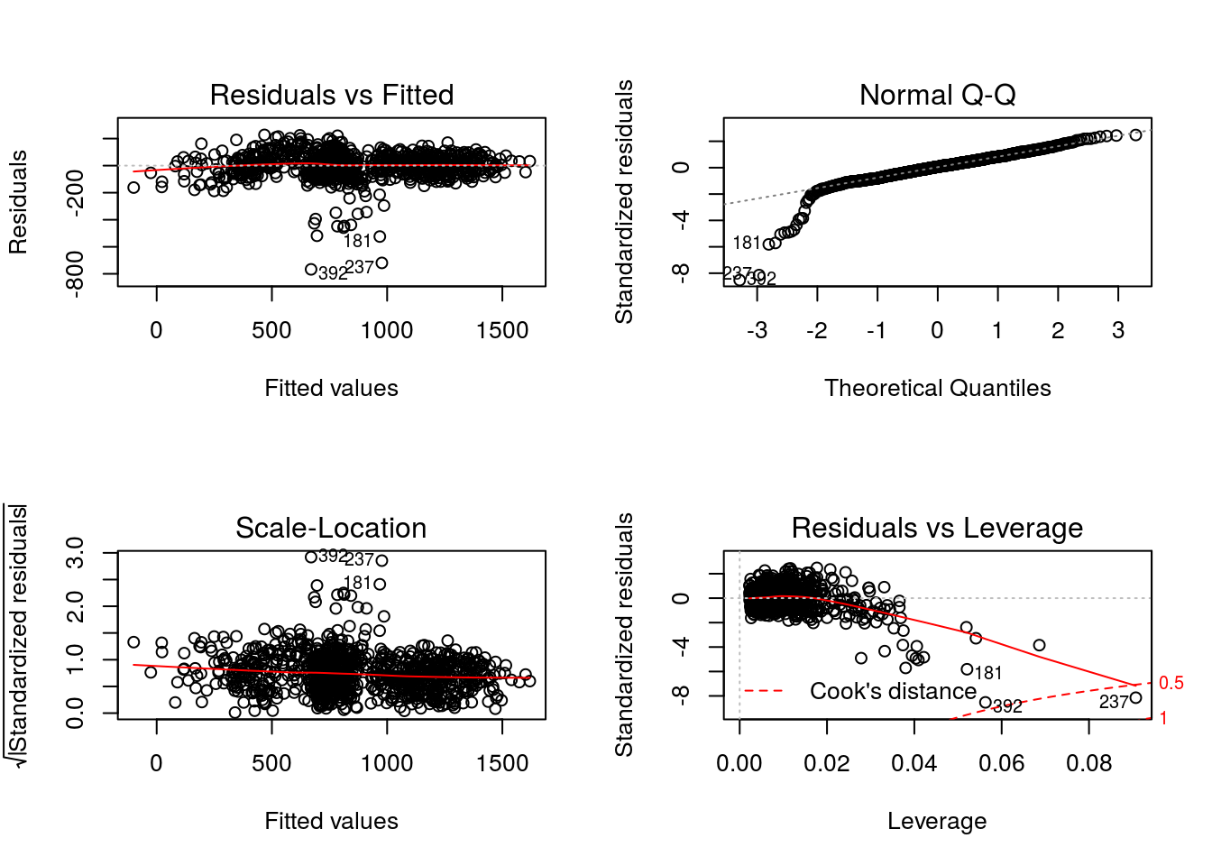

The non-normality seen in the Normal Q-Q plot and the presence of outliers in the Residuals vs Leverage plot are consistent with the fact that this model is misspecified.

The methods discussed in this chapter use the backward iterative algorithm to obtain parameter estimates for the Q-function models. Thus, the pseudo-outcome is used in the second stage regression that follows. Recall, the pseudo-outcome at this decision point is an individuals expected outcome had they received treatment according the optimal treatment regime at Decision 3. The optimal regime is that which maximizes the Q-function, and thus we calculate the pseudo-outcome as follows.

A3 <- dataMDP$A3

dataMDP$A3 <- 0L
Q30 <- stats::predict(object = Q3, newdata = dataMDP)
dataMDP$A3 <- 1L
Q31 <- stats::predict(object = Q3, newdata = dataMDP)
dataMDP$A3 <- A3

V3 <- pmax(Q30, Q31)

The posited model for \(Q_{2}(h_{2},a_{2}) = E(V_{3}(H_{3})|H_{2} = h_{2}, A_{2} = a_{2})\) is misspecified as

\[ \begin{align} Q_{2}(h_{2},a_{2};\beta_{2}) =& \beta_{20} + \beta_{21} \text{CD4_0} + a_{1}~(\beta_{22} + \beta_{23} \text{CD4_0}) \\ & + \beta_{24} \text{CD4_6} + a_{2}~(\beta_{25} + \beta_{26} \text{CD4_6}). \end{align} \]

Modeling Object

The parameters of this model will be estimated using ordinary least squares via R’s stats::lm() function. Predictions will be made using stats::predict.lm(), which by default returns predictions on the scale of the response variable.

The modeling objects for this regression step is

q2 <- modelObj::buildModelObj(model = ~ CD4_0*A1 + CD4_6*A2,
                              solver.method = 'lm',
                              predict.method = 'predict.lm')

Model Diagnostics

Recall that \(Q_{2}(h_{2},a_{2})\) is the expectation of the value, \(V_{3}(H_{3})\); we use the results discussed in the previous regression analysis. For \(Q_{2}(h_{2},a_{2};{\beta}_{2})\) the regression can be completed as follows

Q2 <- modelObj::fit(object = q2, data = dataMDP, response = V3)
Q2 <- modelObj::fitObject(object = Q2)
Q2

Call:
lm(formula = YinternalY ~ CD4_0 + A1 + CD4_6 + A2 + CD4_0:A1 + 
    CD4_6:A2, data = data)

Coefficients:
(Intercept)        CD4_0           A1        CD4_6           A2     CD4_0:A1     CD4_6:A2  
   399.0351       0.9874     447.7761       0.4784     538.3843      -1.8782      -1.6455  

where for convenience we have again made use of modelObj’s fitObject() function to strip away the modeling object framework making Q2 an object of class “lm.”

Let’s examine the diagnostic plots defined for “lm” objects.

par(mfrow = c(2,2))
graphics::plot(x = Q2)

The presence of cases with large residuals in the Residuals vs Fitted plot, the non-normality behavior seen in the Normal Q-Q plot, and the presence of cases beyond the Cook’s distance in the Residuals vs Leverage plot are all consistent with the fact that this model is misspecified.

The methods discussed in this chapter use the backward iterative algorithm to obtain parameter estimates for the Q-function models. Thus, the pseudo-outcome is used in the first stage regression that follows. Recall, the pseudo-outcome at this decision point is an individuals expected outcome had they received treatment according the optimal treatment regime at Decisions 2 and 3. The optimal regime is that which maximizes the Q-function, and thus we calculate the pseudo-outcome as follows.

A2 <- dataMDP$A2

dataMDP$A2 <- 0L
Q20 <- stats::predict(object = Q2, newdata = dataMDP)
dataMDP$A2 <- 1L
Q21 <- stats::predict(object = Q2, newdata = dataMDP)
dataMDP$A2 <- A2

V2 <- pmax(Q20, Q21)

The posited model for \(Q_{1}(h_{1},a_{1}) = E(V_{2}(H_{2})|H_{1} = h_{1}, A_{1} = a_{1})\) is misspecified as,

\[ Q_{1}(h_{1},a_{1};\beta_{1}) = \beta_{10} + \beta_{11} \text{CD4_0} + a_{1}~(\beta_{12} + \beta_{13} \text{CD4_0}). \]

Modeling Object

The parameters of this model will be estimated using ordinary least squares via R’s stats::lm() function. Predictions will be made using stats::predict.lm(), which by default returns predictions on the scale of the response variable.

The modeling objects for this regression step is

q1 <- modelObj::buildModelObj(model = ~ CD4_0*A1,
                              solver.method = 'lm',
                              predict.method = 'predict.lm')

Model Diagnostics

Recall that \(Q_{1}(h_{1},a_{1})\) is the expectation of the value, \(V_{2}(H_{2})\); we use the results discussed in the previous regression analysis. For \(Q_{1}(h_{1},a_{1};\beta_{1})\) the regression can be completed as follows

Q1 <- modelObj::fit(object = q1, data = dataMDP, response = V2)
Q1 <- modelObj::fitObject(object = Q1)
Q1

Call:
lm(formula = YinternalY ~ CD4_0 + A1 + CD4_0:A1, data = data)

Coefficients:
(Intercept)        CD4_0           A1     CD4_0:A1  
    438.800        1.506      465.621       -1.928  

where for convenience we have again made use of modelObj’s fitObject() function to strip away the modeling object framework making Q1 an object of class “lm.”

Let’s examine the diagnostic plots defined for “lm” objects.

par(mfrow = c(2,2))
graphics::plot(x = Q1)

The presence of cases with large residuals in the Residuals vs Fitted plot, the non-normality behavior seen in the Normal Q-Q plot, and the presence of cases beyond the Cook’s distance in the Residuals vs Leverage plot are all consistent with the fact that this model is misspecified.

\(\pi_{k}(h_{k};\gamma_{k})\)

To streamline the presentation of methods, we consider only one propensity score model for each decision point. Note that we are not demonstrating a definitive analysis that one might do in practice, in which the analyst would use all sorts of variable selection techniques, etc., to arrive at a posited model. Our objective is to illustrate how to apply the methods; we have chosen to use the data generating models, which are a class of models that are likely to be familiar to many readers and will not obfuscate the objective.

Click on each tab below to see each model and basic model diagnostic steps.

• \(\pi_{1}(h_{1};\gamma_{1})\)
• \(\pi_{2}(h_{2};\gamma_{2})\)
• \(\pi_{3}(h_{3};\gamma_{3})\)

The posited model for the first decision point is the model used to generate the data

\[ \pi_{1}(h_{1};\gamma_{1}) = \frac{\exp(\gamma_{10} + \gamma_{11}~\text{CD4_0})}{1+\exp(\gamma_{10} + \gamma_{11}~\text{CD4_0})}. \]

Modeling Object

The parameters of this model will be estimated using maximum likelihood via R’s stats::glm() function. Predictions will be made using stats::predict.glm(), which by default returns predictions on the scale of the linear predictors. For methods implemented in DynTxRegime, prediction for the propensity score must always be on the scale of the response variable, i.e., the probabilities. The modeling object for this model is specified as

p1 <- modelObj::buildModelObj(model = ~ CD4_0,
                              solver.method = 'glm',
                              solver.args = list(family='binomial'),
                              predict.method = 'predict.glm',
                              predict.args = list(type='response'))

Model Diagnostics

Though the estimators are implemented in DynTxRegime such that the regression step is performed internally and model diagnostics can be performed post-analysis, it is convenient to do model diagnostics separately here. We will make use of modelObj::fit() to complete the regression step.

For \(\pi_{1}(h_{1};\gamma)\) the regression can be completed as follows:

PS1 <- modelObj::fit(object = p1, data = dataMDP, response = dataMDP$A1)
PS1 <- modelObj::fitObject(object = PS1)
PS1

Call:  glm(formula = YinternalY ~ CD4_0, family = "binomial", data = data)

Coefficients:
(Intercept)        CD4_0  
   2.356590    -0.006604  

Degrees of Freedom: 999 Total (i.e. Null);  998 Residual
Null Deviance:      1315 
Residual Deviance: 1228     AIC: 1232

where for convenience we have made use of modelObj’s fitObject() function to strip away the modeling object framework making PS1 an object of class “glm.”

Though we know this model to be correctly specified, let’s examine the regression results.

summary(object = PS1)

Call:
glm(formula = YinternalY ~ CD4_0, family = "binomial", data = data)

Deviance Residuals: 
    Min       1Q   Median       3Q      Max  
-1.9010  -0.9414  -0.7107   1.2178   2.1054  

Coefficients:
              Estimate Std. Error z value Pr(>|z|)    
(Intercept)  2.3565904  0.3353980   7.026 2.12e-12 ***
CD4_0       -0.0066038  0.0007588  -8.703  < 2e-16 ***
---
Signif. codes:  0 '***' 0.001 '**' 0.01 '*' 0.05 '.' 0.1 ' ' 1

(Dispersion parameter for binomial family taken to be 1)

    Null deviance: 1314.7  on 999  degrees of freedom
Residual deviance: 1227.6  on 998  degrees of freedom
AIC: 1231.6

Number of Fisher Scoring iterations: 4

In comparing the null deviance (1314.7) and the residual deviance (1227.6), we see that including the independent variable, \(\text{CD4_0}\), reduces the deviance relative to the simpler constant propensity score model. This result is consistent with the fact that it is the model used to generate our data.

The posited model for the second decision point is the model used to generate the data

\[ \pi_{2}(h_{2};\gamma_{2}) = \frac{\exp(\gamma_{20} + \gamma_{21}~\text{CD4_6})}{1+\exp(\gamma_{20} + \gamma_{21}~\text{CD4_6})}. \]

Modeling Object

The parameters of this model will be estimated using maximum likelihood via R’s stats::glm() function. Predictions will be made using stats::predict.glm(), which by default returns predictions on the scale of the linear predictors. For methods implemented in DynTxRegime, prediction for the propensity score must always be on the scale of the response variable, i.e., the probabilities. The modeling object for this model is specified as

p2 <- modelObj::buildModelObj(model = ~ CD4_6,
                              solver.method = 'glm',
                              solver.args = list(family='binomial'),
                              predict.method = 'predict.glm',
                              predict.args = list(type='response'))

Model Diagnostics

Though the estimators are implemented in DynTxRegime such that the regression step is performed internally and model diagnostics can be performed post-analysis, it is convenient to do model diagnostics separately here. We will make use of modelObj::fit() to complete the regression step.

For \(\pi_{2}(h_{2};\gamma_{2})\) the regression can be completed as follows:

PS2 <- modelObj::fit(object = p2, data = dataMDP, response = dataMDP$A2)
PS2 <- modelObj::fitObject(object = PS2)
PS2

Call:  glm(formula = YinternalY ~ CD4_6, family = "binomial", data = data)

Coefficients:
(Intercept)        CD4_6  
   0.818685    -0.004294  

Degrees of Freedom: 999 Total (i.e. Null);  998 Residual
Null Deviance:      951.8 
Residual Deviance: 911.4    AIC: 915.4

where for convenience we have made use of modelObj’s fitObject() function to strip away the modeling object framework making PS2 an object of class “glm.”

Though we know this model to be correctly specified, let’s examine the regression results.

summary(object = PS2)

Call:
glm(formula = YinternalY ~ CD4_6, family = "binomial", data = data)

Deviance Residuals: 
    Min       1Q   Median       3Q      Max  
-1.2416  -0.6751  -0.5610  -0.4157   2.2830  

Coefficients:
              Estimate Std. Error z value Pr(>|z|)    
(Intercept)  0.8186852  0.3733067   2.193   0.0283 *  
CD4_6       -0.0042941  0.0006989  -6.144 8.05e-10 ***
---
Signif. codes:  0 '***' 0.001 '**' 0.01 '*' 0.05 '.' 0.1 ' ' 1

(Dispersion parameter for binomial family taken to be 1)

    Null deviance: 951.82  on 999  degrees of freedom
Residual deviance: 911.44  on 998  degrees of freedom
AIC: 915.44

Number of Fisher Scoring iterations: 4

In comparing the null deviance (951.8) and the residual deviance (911.4), we see that including the independent variable, \(\text{CD4_6}\) reduces the deviance relative to the simpler constant propensity score model. This result is consistent with the fact that it is the model used to generate our data.

The posited model for the final decision point is the model used to generate the data

\[ \pi_{3}(h_{3};\gamma_{3}) = \frac{\exp(\gamma_{30} + \gamma_{31}~\text{CD4_12})}{1+\exp(\gamma_{30} + \gamma_{31}~\text{CD4_12})}. \]

Modeling Object

The parameters of this model will be estimated using maximum likelihood via R’s stats::glm() function. Predictions will be made using stats::predict.glm(), which by default returns predictions on the scale of the linear predictors. For methods implemented in DynTxRegime, prediction for the propensity score must always be on the scale of the response variable, i.e., the probabilities. The modeling object for this model is specified as

p3 <- modelObj::buildModelObj(model = ~ CD4_12,
                              solver.method = 'glm',
                              solver.args = list(family='binomial'),
                              predict.method = 'predict.glm',
                              predict.args = list(type='response'))

Model Diagnostics

Though the estimators are implemented in DynTxRegime such that the regression step is performed internally and model diagnostics can be performed post-analysis, it is convenient to do model diagnostics separately here. We will make use of modelObj::fit() to complete the regression step.

For \(\pi_{3}(h_{3};\gamma_{3})\) the regression can be completed as follows:

PS3 <- modelObj::fit(object = p3, data = dataMDP, response = dataMDP$A3)
PS3 <- modelObj::fitObject(object = PS3)
PS3

Call:  glm(formula = YinternalY ~ CD4_12, family = "binomial", data = data)

Coefficients:
(Intercept)       CD4_12  
   1.411752    -0.004945  

Degrees of Freedom: 999 Total (i.e. Null);  998 Residual
Null Deviance:      1252 
Residual Deviance: 1203     AIC: 1207

where for convenience we have made use of modelObj’s fitObject() function to strip away the modeling object framework making PS3 an object of class “glm.”

Though we know this model to be correctly specified, let’s examine the regression results.

summary(object = PS3)

Call:
glm(formula = YinternalY ~ CD4_12, family = "binomial", data = data)

Deviance Residuals: 
    Min       1Q   Median       3Q      Max  
-1.4176  -0.9026  -0.7373   1.2970   2.0555  

Coefficients:
             Estimate Std. Error z value Pr(>|z|)    
(Intercept)  1.411752   0.324038   4.357 1.32e-05 ***
CD4_12      -0.004945   0.000734  -6.736 1.62e-11 ***
---
Signif. codes:  0 '***' 0.001 '**' 0.01 '*' 0.05 '.' 0.1 ' ' 1

(Dispersion parameter for binomial family taken to be 1)

    Null deviance: 1252.2  on 999  degrees of freedom
Residual deviance: 1203.0  on 998  degrees of freedom
AIC: 1207

Number of Fisher Scoring iterations: 4

In comparing the null deviance (1252.2) and the residual deviance (1203), we see that including the independent variable, \(\text{CD4_12}\), reduces the deviance relative to the simpler constant propensity score model. This result is consistent with the fact that it is the model used to generate our data.

• Value of a Fixed Regime
• R Codes