
Q-learning
The Q-learning algorithm was introduced previously in Chapter 5. We repeat it here with modifcation for \(\Psi\)-specific regimes.
An optimal \(\Psi\)-specific regime \(d^{opt}\) can be represented in terms of Q-functions
\[ Q_{K}(h_{K},a_{K}) = Q_{K}(\overline{x}_{K},\overline{a}_{K}) = E(Y|\overline{X} = \overline{x}, \overline{A} = \overline{a}) \]
and for \(k = K-1, \dots, 1\)
\[ Q_{k}(h_{k},a_{k}) = Q_{k}(\overline{x}_{k},\overline{a}_{k}) = E\{ V_{k+1}(\overline{x}_{k},X_{k+1},\overline{a}_{k}) |\overline{X}_{k} = \overline{x}_{k}, \overline{A}_{k} = \overline{a}_{k}\}, \] where for \(k = 1, \dots, K\),
\[ V_{k}(h_{k}) = V_{k}(\overline{x}_k,\overline{a}_{k-1}) = \max_{a_{k} \in \Psi_{k}(h_{k})} Q_{k}(h_{k},a_{k}). \]
Estimation of \(d^{opt}\) via Q-learning is accomplished by positing models for the Q-functions \(Q_{k}(h_{k},a_{k})\),
\[ Q_{k}(h_{k},a_{k};\beta_{k}) = Q_{k}(\overline{x}_{k}, \overline{a}_{k}; \beta_{k}), \quad k = K, K-1, \dots, 1. \]
Estimators \(\widehat{\beta}_{k}\) for \(\beta_{k}\) are obtained in a backward iterative fashion for \(k=K,K-1,\ldots,1\) by solving suitable M-estimating equations.
The estimated rules for \(k = 1, \dots, K\) are \[ \widehat{d}^{opt}_{Q,k}(h_{k}) = d^{opt}_{k}(h_{k};\widehat{\beta}_{k}) = \underset{a_{k} \in \Psi_{k}(h_{k})}{\arg\!\max} ~ Q_{k}(h_{k}, a_{k};\widehat{\beta}_{k}), \] and the pseudo outcomes are \[ \tilde{V}_{ki} = \underset{a_{k} \in \Psi_{k}(h_{k})}{\max} ~ Q_{k}(h_{k}, a_{k};\widehat{\beta}_{k}). \]
An estimated optimal \(\Psi\)-specific regime is then given by
\[
\widehat{d}^{opt}_{Q} = \{\widehat{d}^{opt}_{Q,1}(h_{1}), \dots, \widehat{d}^{opt}_{Q,K}(h_{K})\}
\] and an estimator for the value \(\mathcal{V}(d^{opt})\) is given by \[
\widehat{\mathcal{V}}_{Q}(d^{opt}) = n^{-1} \sum_{i=1}^{n} \tilde{V}_{1i} = n^{-1} \sum_{i=1}^{n} \underset{a_{1} \in \Psi_{1}(H_{1i})}{\max} ~ Q_{1}(H_{1i}, a_{1};\widehat{\beta}_{1}).
\]
A general implementation of the steps of the Q-learning algorithm is provided in
A general implementation of the Q-learning algorithm is provided in
The function call for DynTxRegime::
utils::str(object = DynTxRegime::qLearn)function (..., moMain, moCont, data, response, txName, fSet = NULL, iter = 0L, verbose = TRUE) We briefly describe the input arguments for DynTxRegime::
| Input Argument | Description |
|---|---|
| \(\dots\) | Ignored; included only to require named inputs. |
| moMain | A “modelObj” object or a list of “modelObj” objects. The modeling object(s) for the \(\nu_{k}(h_{k}; \phi_{k})\) component of \(Q_{k}(h_{k},a_{k};\beta_{k})\). |
| moCont | A “modelObj” object or a list of “modelObj” objects. The modeling object(s) for the \(\text{C}_{k}(h_{k}; \psi_{k})\) component of \(Q_{k}(h_{k},a_{k};\beta_{k})\). |
| data | A “data.frame” object. The covariate history and the treatments received. |
| response | For Decision K analysis, a “numeric” vector. The outcome of interest, where larger values are better. For analysis of Decision k, k = 1, …, K-1, a “QLearn” object. The value object returned by |
| txName | A “character” object. The column header of data corresponding to the \(k^{th}\) stage treatment variable. |
| fSet | A “function”. A user defined function specifying treatment or model subset structure of Decision \(k\). |
| iter | An “integer” object. The maximum number of iterations for iterative algorithm. |
| verbose | A “logical” object. If TRUE progress information is printed to screen. |
Methods implemented in DynTxRegime break the Q-function model into two components: a main effects component and a contrasts component. For example, for binary treatments, \(Q_{k}(h_{k}, a_{k}; \beta_{k})\) can be written as
\[ Q_{k}(h_{k}, a_{k}; \beta_{k})= \nu_{k}(h_{k}; \phi_{k}) + a_{k} \text{C}_{k}(h_{k}; \psi_{k}), \text{for} ~ k = 1, \dots, K \]
where \(\beta_{k} = (\phi^{\intercal}_{k}, \psi^{\intercal}_{k})^{\intercal}\). Here, \(\nu_{k}(h_{k}; \phi_{k})\) comprises the terms of the model that are independent of treatment (so called “main effects” or “common effects”), and \(\text{C}_{k}(h_{k}; \psi_{k})\) comprises the terms of the model that interact with treatment (so called “contrasts”). Input arguments moMain and moCont specify \(\nu_{k}(h_{k}; \phi_{k})\) and \(\text{C}_{k}(h_{k}; \psi_{k})\), respectively.
In the examples provided in this chapter, the two components of each \(Q_{k}(h_{k}, a_{k}; \beta_{k})\) are both linear models, the parameters of which are estimated using stats::
Input fSet is a user-defined function specifying the feasible sets. The only requirements for this input are:
- The formal input argument(s) of the function must be either data or the individual covariates required for identifying subset membership.
- The function must return a list containing two elements $subsets and $txOpts.
Element $subsets of the returned list is itself a list; each element of the list contains a nickname and the treatment options for a single feasible set.
Element $txOpts of the returned list is a character vector providing the nickname of the feasible set to which each individual is assigned. - There are no requirements for the function name or the structure of the function contents.
See the Analysis tab for explicit examples.
The value object returned by DynTxRegime::
| Slot Name | Description |
|---|---|
| @step | The step of the Q-learning algorithm to which this object pertains. |
| @analysis@outcome | The Q-function regression analysis. |
| @analysis@txInfo | The treatment information. |
| @analysis@call | The unevaluated function call. |
| @analysis@optimal | The estimated value, Q-functions, and optimal treatment for the training data. |
There are several methods available for objects of this class that assist with model diagnostics, the exploration of training set results, and the estimation of optimal treatments for future patients. We explore some of these methods in the Methods section.
The Q-learning algorithm begins with the analysis of Decision \(K\). In our current example, \(K=3\).
Inputs moMain and moCont are modeling objects specifying the model posited for \(Q_{3}(h_3, a_3) = E(Y|\overline{X} = \overline{x}, \overline{A} = \overline{a})\). We posit the following model
\[ Q_{3}(h_{3},a_{3};{\beta}_{3}) = {\beta}_{30} + {\beta}_{31} \text{CD4_0} + {\beta}_{32} \text{CD4_6} + {\beta}_{33} \text{CD4_12} + a_{3}~({\beta}_{34} + {\beta}_{35} \text{CD4_12}), \]
the modeling objects of which are specified as
q3Main <- modelObj::buildModelObj(model = ~ CD4_0 + CD4_6 + CD4_12,
                                  solver.method = 'lm',
                                  predict.method = 'predict.lm')
q3Cont <- modelObj::buildModelObj(model = ~ CD4_12,
solver.method = 'lm',
predict.method = 'predict.lm')Note that the formula in the contrast component q3Cont does not contain the third stage treatment variable; it contains only the covariate(s) that interact with the treatment.
Both components of the outcome regression model are of the same class, and the models should be fit as a single combined object. Thus, the iterative algorithm is not required, and iter=0, its default value.
To see a brief synopsis of the model diagnostics for this model, see header \(Q_{k}(h_{k},a_{k};\beta_{k})\) in the sidebar menu.
The “data.frame” containing all covariates and treatments received is data set dataMDPF, the third stage treatment is contained in column $A3 of this data set, and the outcome of interest for the first step of the Q-learning algorithm is $Y of dataMDPF.
Because not all treatments are available to all patients, we must define fSet, a function that defines the feasible sets and matches individuals to the appropriate feasible set. Specifically, the feasible sets for Decision 3 are defined to be
\[ \Psi_{3}(h_{3}) = \left\{ \begin{array}{cl} \{1\} \subset \mathcal{A}_{3} & \text{if } A_{2} = 1~\{s_{3}(h_{3}) = 1\}\\ \{ 0,1\} \subset \mathcal{A}_{3}& \text{if } A_{2} = 0~\{s_{3}(h_{3}) = 2\}\\ \end{array} \right. . \]
That is, individuals that received treatment \(A_{2}=1\) remain on treatment 1. All others are assigned one of \(A_{3} = \{0,1\}\). An example of a user-defined function that defines the feasible sets for Decision 3 is
fSet3 <- function(data){
           subsets <- list(list("s1",1L),
                           list("s2",c(0L,1L)))

           txOpts <- rep(x = 's2', times = nrow(x = data))
           txOpts[data$A2 == 1L] <- "s1"

           return(list("subsets" = subsets, "txOpts" = txOpts))
         }
Note that this is not the only possible function specification; there are innumerable ways to specify this rule in R. The only requirements for this input are that the formal input argument of the function must be data and that the function must return a list containing $subsets and $txOpts, which contain a list describing the feasible sets and a vector specifying the feasible set to which each patient is associated.
The optimal treatment rule for Decision 3, \(\widehat{d}_{Q,3}^{opt}(h_{3})\), is estimated as follows.
QL3 <- DynTxRegime::qLearn(moMain = q3Main,
                           moCont = q3Cont,
                           data = dataMDPF,
                           response = dataMDPF$Y,
                           txName = 'A3',
                           fSet = fSet3,
                           verbose = TRUE)
First step of the Q-Learning Algorithm.
Subsets of treatment identified as:
$s1
[1] 1
$s2
[1] 0 1
Number of patients in data for each subset:
s1 s2
486 514
Outcome regression.NOTE: subset(s) s1 excluded from outcome regressionCombined outcome regression model: ~ CD4_0+CD4_6+CD4_12 + A3 + A3:(CD4_12) .
514 included in analysis
Regression analysis for Combined:
Call:
lm(formula = YinternalY ~ CD4_0 + CD4_6 + CD4_12 + A3 + CD4_12:A3,
data = data)
Coefficients:
(Intercept) CD4_0 CD4_6 CD4_12 A3 CD4_12:A3
317.3743 2.0326 0.1371 -0.4478 603.5614 -1.9814
Recommended Treatments:
0 1
502 498
Estimated value: 951.8159 Above, we opted to set verbose to TRUE to highlight some of the information that should be verified by a user. Notice the following:
- The first line of the verbose output indicates that the analysis is the first step of the Q-learning algorithm.
Users should verify that this is the intended step. - The feasible sets are summarized including the number of individuals assigned to each set.
Users should verify that input fSet was properly interpreted by the software. - The information provided for the Q-function (outcome) regression is not defined within DynTxRegime::
qLearn() , but is specified by the statistical method selected to obtain parameter estimates; in this example it is defined by stats::lm() .
Users should verify that the model was correctly interpreted by the software and that there are no warnings or messages reported by the regression method. - Notice that only a subset of the data was used in the outcome regression analysis. This reflects that only those individuals for whom more than one treatment option was available were included in the regression, i.e., only those for whom \(s_{3}(h_{3}) = 2\).
- Finally, a tabled summary of the recommended treatments and the estimated value for the training data are shown.
Recall that this estimated value is not the estimated value of the full optimal regime, but is the mean of the pseudo-outcomes \(\tilde{V}_{3}\).
The first step of the post-analysis should always be model diagnostics. DynTxRegime comes with several tools to assist in this task. However, we have explored the propensity score and Q-function models previously and will skip that step here. A review of those models can be found through the respective links in the sidebar.
For individuals for whom \(s_{3}(h_{3}) = 2\), the form of the regression model dictates the class of regimes under consideration. For \(Q_{3}(h_{3},a_{3};{\beta}_{3})\) the regime is of the form
\[ \widehat{d}_{Q,3}^{opt}(h_{3}) = a_{2} + (1-a_{2})~\text{I}(\widehat{\beta}_{34} + \widehat{\beta}_{35} \text{CD4_12} > 0). \]
The parameter estimates, \(\widehat{\beta}_{3}\), can be retrieved using DynTxRegime::
DynTxRegime::coef(object = QL3)$outcome
$outcome$Combined
(Intercept) CD4_0 CD4_6 CD4_12 A3 CD4_12:A3
317.3743233 2.0326241 0.1371394 -0.4477942 603.5613540 -1.9814314 and thus \[ \begin{align} \widehat{d}^{opt}_{Q,3}(h_{3}) &= a_{2} + (1-a_{2})~\text{I} (603.56 - 1.98 ~ \text{CD4_12} > 0) \\ &= a_{2} + (1-a_{2})~\text{I} (\text{CD4_12} < 304.61~\text{cells}/\text{mm}^3). \end{align} \]
There are several methods available for the returned object that assist with model diagnostics, the exploration of training set results, and the estimation of optimal treatments for future patients. A complete description of these methods can be found under the Methods tab.
The second step of the Q-learning algorithm is the analysis of Decision \(K-1 = 2\).
Inputs moMain and moCont are modeling objects specifying the model posited for \(Q_{2}(h_2, a_2) = E\{V_{3}(\overline{x}_{2},X_{3},\overline{a}_2)|\overline{X}_2 = \overline{x}_2, \overline{A}_2 = \overline{a}_2\}\). We posit the following model
\[ Q_{2}(h_{2},a_{2};\beta_{2}) = \beta_{20} + \beta_{21} \text{CD4_0} + \beta_{22} \text{CD4_6} + a_{2}~(\beta_{23} + \beta_{24} \text{CD4_6}), \]
the modeling objects of which are specified as
q2Main <- modelObj::buildModelObj(model = ~ CD4_0 + CD4_6,
                                  solver.method = 'lm',
                                  predict.method = 'predict.lm')
q2Cont <- modelObj::buildModelObj(model = ~ CD4_6,
solver.method = 'lm',
predict.method = 'predict.lm')Note that the formula in the contrast component q2Cont does not contain the third stage treatment variable; it contains only the covariate(s) that interact with the treatment.
Both components of the outcome regression model are of the same class, and the models should be fit as a single combined object. Thus, the iterative algorithm is not required, and iter=0, its default value.
To see a brief synopsis of the model diagnostics for this model, see header \(Q_{k}(h_{k},a_{k};\beta_{k})\) in the sidebar menu.
The “data.frame” containing all covariates and treatments received is data set dataMDPF and the second stage treatment is contained in column $A2 of this data set. Because this step is a continuation step of the Q-learning algorithm, response is the value object returned by step 1, QL3<>.
Because not all treatments are available to all patients, we must define fSet, a function that defines the feasible sets and matches individuals to the appropriate feasible set. Specifically, the feasible sets for Decision 2 are defined to be
\[ \Psi_{2}(h_{2}) = \left\{ \begin{array}{cl} \{1\} \subset \mathcal{A}_{2} & \text{if } A_{1} = 1 ~\{s_{2}(h_{2}) = 1\}\\ \{ 0,1\} \subset \mathcal{A}_{2}& \text{if } A_{1} = 0~\{s_{2}(h_{2}) = 2\}\\ \end{array} \right. . \]
That is, individuals that received treatment \(A_{1}=1\) remain on treatment 1. All others are assigned one of \(A_{2} = \{0,1\}\). An example of a user-defined function that defines the feasible sets for Decision 2 is
fSet2 <- function(data){
           subsets <- list(list("s1",1L),
                           list("s2",c(0L,1L)))

           txOpts <- rep(x = 's2', times = nrow(x = data))
           txOpts[data$A1 == 1L] <- "s1"

           return(list("subsets" = subsets, "txOpts" = txOpts))
         }
Note that this is not the only possible function specification; there are innumerable ways to specify this rule in R. The only requirements for this input are that the formal input argument of the function must be data and that the function must return a list containing $subsets and $txOpts, which contain a list describing the feasible sets and a vector specifying the feasible set to which each patient is associated.
The optimal treatment rule for Decision 2, \(\widehat{d}_{Q,2}^{opt}(h_{2})\), is estimated as follows.
QL2 <- DynTxRegime::qLearn(moMain = q2Main,
                           moCont = q2Cont,
                           data = dataMDPF,
                           response = QL3,
                           txName = 'A2',
                           fSet = fSet2,
                           verbose = TRUE)
Step 2 of the Q-Learning Algorithm.
Subsets of treatment identified as:
$s1
[1] 1
$s2
[1] 0 1
Number of patients in data for each subset:
s1 s2
368 632
Outcome regression.NOTE: subset(s) s1 excluded from outcome regressionCombined outcome regression model: ~ CD4_0+CD4_6 + A2 + A2:(CD4_6) .
632 included in analysis
Regression analysis for Combined:
Call:
lm(formula = YinternalY ~ CD4_0 + CD4_6 + A2 + CD4_6:A2, data = data)
Coefficients:
(Intercept) CD4_0 CD4_6 A2 CD4_6:A2
344.9733 1.8566 -0.1238 500.7085 -1.6028
Recommended Treatments:
0 1
624 376
Estimated value: 994.5354 The verbose output generated is very similar to that of step 1. Notice, however, that the first line of the verbose output indicates that this analysis is “Step 2.” Users should verify that this is the intended step. If it is not, verify input response. As mentioned in step 1, the estimated value is not the estimated value of the full optimal regime but is the mean of the pseudo-outcomes \(\tilde{V}_{2}\). As seen in the previous step, only a subset of the data was used in the outcome regression analysis. This reflects that only those individuals for whom more than one treatment option was available were included in the regression, i.e., only those for whom \(s_{2}(h_{2}) = 2\).
The first step of the post-analysis should always be model diagnostics. DynTxRegime comes with several tools to assist in this task. However, we have explored the propensity score and Q-function models previously and will skip that step here. A review of those models can be found through the respective links in the sidebar.
For individuals for whom \(s_{2}(h_{2}) = 2\), the form of the regression model dictates the class of regimes under consideration. For \(Q_{2}(h_{2},a_{2};{\beta}_{2})\) the regime is of the form
\[ \widehat{d}_{Q,2}^{opt}(h_{2}) = a_{1} + (1-a_{1})~\text{I}(\widehat{\beta}_{23} + \widehat{\beta}_{24} \text{CD4_6} > 0). \]
The parameter estimates, \(\widehat{\beta}_{2}\), can be retrieved using DynTxRegime::
DynTxRegime::coef(object = QL2)$outcome
$outcome$Combined
(Intercept) CD4_0 CD4_6 A2 CD4_6:A2
344.9732599 1.8565589 -0.1238184 500.7085250 -1.6027885 and thus \[ \begin{align} \widehat{d}^{opt}_{Q,2}(h_{2}) &= a_{1} + (1-a_{1})~\text{I} (500.71 - 1.60 ~ \text{CD4_6} > 0) \\ &= a_{1} + (1-a_{1})~\text{I} (\text{CD4_6} < 312.40~\text{cells}/\text{mm}^3). \end{align} \]
There are several methods available for the returned object that assist with model diagnostics, the exploration of training set results, and the estimation of optimal treatments for future patients. A complete description of these methods can be found under the Methods tab.
The final step of the Q-learning algorithm is the analysis of Decision \(k = 1\).
Inputs moMain and moCont are modeling objects specifying the model posited for \(Q_{1}(h_1, a_1) = E\{V_{2}(x_{1},X_{2},a_{1})|X_{1} = x_{1}, A_{1} = a_{1}\}\). We posit the following model
\[ Q_{1}(h_{1},a_{1};\beta_{1}) = \beta_{10} + \beta_{11} \text{CD4_0} + a_{1}~(\beta_{12} + \beta_{13} \text{CD4_0}), \]
the modeling objects of which are specified as
q1Main <- modelObj::buildModelObj(model = ~ CD4_0,
                                  solver.method = 'lm',
                                  predict.method = 'predict.lm')
q1Cont <- modelObj::buildModelObj(model = ~ CD4_0,
solver.method = 'lm',
predict.method = 'predict.lm')Note that the formula in the contrast component q1Cont does not contain the third stage treatment variable; it contains only the covariate(s) that interact with the treatment.
Both components of the outcome regression model are of the same class, and the models should be fit as a single combined object. Thus, the iterative algorithm is not required, and iter=0, its default value.
To see a brief synopsis of the model diagnostics for this model, see header \(Q_{k}(h_{k},a_{k};\beta_{k})\) in the sidebar menu.
The “data.frame” containing all covariates and treatments received is data set dataMDPF and the first stage treatment is contained in column $A1 of this data set. Because this step is a continuation step of the Q-learning algorithm, response is the value object returned by step 2, QL2.
Because there is only one feasible set for all individuals at this decision point, fSet is kept at its default value, NULL.
The optimal treatment rule for Decision 1, \(\widehat{d}_{Q,1}^{opt}(h_{1})\), is estimated as follows.
QL1 <- DynTxRegime::qLearn(moMain = q1Main,
                           moCont = q1Cont,
                           data = dataMDPF,
                           response = QL2,
                           txName = 'A1',
                           fSet = NULL,
                           verbose = TRUE)
Step 3 of the Q-Learning Algorithm.
Outcome regression.
Combined outcome regression model: ~ CD4_0 + A1 + A1:(CD4_0) .
Regression analysis for Combined:
Call:
lm(formula = YinternalY ~ CD4_0 + A1 + CD4_0:A1, data = data)
Coefficients:
(Intercept) CD4_0 A1 CD4_0:A1
379.564 1.632 477.623 -1.932
Recommended Treatments:
0 1
979 21
Estimated value: 1112.179 The verbose output generated is very similar to that of steps 1 and 2. However, the first line of the verbose output indicates that this analysis is “Step 3.” Users should verify that this is the intended step. If it is not, verify input response. There is no way to indicate to the software that this is the “final” step of the algorithm.
The first step of the post-analysis should always be model diagnostics. DynTxRegime comes with several tools to assist in this task. However, we have explored the propensity score and Q-function models previously and will skip that step here. A review of those models can be found through the respective links in the sidebar.
As for the previous steps, the form of the regression model dictates the class of regimes under consideration. For model \(Q_{1}(h_{1},a_{1};\beta_{1})\) the regime is of the form
\[ \widehat{d}_{Q,1}^{opt}(h_{1}) = \text{I}(\widehat{\beta}_{12} + \widehat{\beta}_{13} \text{CD4_0} > 0). \]
The parameter estimates, \(\widehat{\beta}_{1}\) can be retrieved using DynTxRegime::
DynTxRegime::coef(object = QL1)$outcome
$outcome$Combined
(Intercept) CD4_0 A1 CD4_0:A1
379.563861 1.632416 477.623381 -1.931750 and thus \[ \begin{align} \widehat{d}^{opt}_{Q,1}(h_{1}) &= \text{I} (477.62 - 1.93 ~\text{CD4_0} > 0) \\ &= \text{I} (\text{CD4_0} < 247.25~\text{cells}/\text{mm}^3). \end{align} \]
The complete estimated optimal treatment regime \(\widehat{d}_{Q}^{opt} = \{\widehat{d}^{opt}_{Q,1}(h_{1}),\widehat{d}^{opt}_{Q,2}(h_{2}),\widehat{d}^{opt}_{Q,3}(h_{3})\}\) is characterized by the following rules
\[ \begin{align} \widehat{d}^{opt}_{Q,1}(h_{1}) &= \text{I} (\text{CD4_0} < 247.25 ~ \text{cells}/\text{mm}^3)\\ \widehat{d}^{opt}_{Q,2}(h_{2}) &= a_{1} + (1-a_{1})\text{I} (\text{CD4_6} < 312.40 ~ \text{cells}/\text{mm}^3)\\ \widehat{d}^{opt}_{Q,3}(h_{3}) &= a_{2} + (1-a_{2})\text{I} (\text{CD4_12} < 304.61 ~ \text{cells}/\text{mm}^3) \end{align} \]
Recall that the rules of the true optimal treatment regime are
\[ \begin{align} d^{opt}_{1}(h_{1}) &= \text{I} (\text{CD4_0} < 250 ~ \text{cells/mm}^3) \\ d^{opt}_{2}(h_{2}) &= d_{1}(h_{1}) + \{1 - d_{1}(h_{1})\} \text{I} (\text{CD4_6} < 360 ~ \text{cells/mm}^3) \\ d^{opt}_{3}(h_{3}) &= d_{2}(h_{2}) + \{1 - d_{2}(h_{2})\} \text{I} (\text{CD4_12} < 300 ~ \text{cells/mm}^3) \end{align} \]
Finally, as this is the last step of the Q-learning algorithm, function DynTxRegime::
DynTxRegime::estimator(x = QL1)[1] 1112.179The true value under the optimal regime, \(\mathcal{V}(d^{opt})\), is \(1120\) cells/mm\(^3\)
Technically, function DynTxRegime::
There are several methods available for the returned object that assist with model diagnostics, the exploration of training set results, and the estimation of optimal treatments for future patients. A complete description of these methods can be found under the Methods tab.
We illustrate the methods available for objects of class “QLearn” by considering the following analysis:
q3Main <- modelObj::buildModelObj(model = ~ CD4_0 + CD4_6 + CD4_12,
                                  solver.method = 'lm',
                                  predict.method = 'predict.lm')
q3Cont <- modelObj::buildModelObj(model = ~ CD4_12,
solver.method = 'lm',
predict.method = 'predict.lm')result3 <- DynTxRegime::qLearn(moMain = q3Main,
moCont = q3Cont,
data = dataMDPF,
response = dataMDPF$Y,
txName = 'A3',
iter = 0L,
fSet = fSet3,
verbose = FALSE)NOTE: subset(s) s1 excluded from outcome regressionq2Main <- modelObj::buildModelObj(model = ~ CD4_0 + CD4_6,
solver.method = 'lm',
predict.method = 'predict.lm')q2Cont <- modelObj::buildModelObj(model = ~ CD4_6,
solver.method = 'lm',
predict.method = 'predict.lm')result2 <- DynTxRegime::qLearn(moMain = q2Main,
moCont = q2Cont,
data = dataMDPF,
response = result3,
txName = 'A2',
iter = 0L,
fSet = fSet2,
verbose = FALSE)NOTE: subset(s) s1 excluded from outcome regressionq1Main <- modelObj::buildModelObj(model = ~ CD4_0,
solver.method = 'lm',
predict.method = 'predict.lm')q1Cont <- modelObj::buildModelObj(model = ~ CD4_0,
solver.method = 'lm',
predict.method = 'predict.lm')result1 <- DynTxRegime::qLearn(moMain = q1Main,
moCont = q1Cont,
data = dataMDPF,
response = result2,
txName = 'A1',
iter = 0L,
fSet = NULL,
verbose = FALSE)| Function | Description |
|---|---|
| Call(name, …) | Retrieve the unevaluated call to the statistical method. |
| coef(object, …) | Retrieve estimated parameters of outcome model(s). |
| DTRstep(object) | Print description of method used to estimate the treatment regime and value. |
| estimator(x, …) | Retrieve the estimated value of the estimated optimal treatment regime for the training data set. |
| fitObject(object, …) | Retrieve the regression analysis object(s) without the modelObj framework. |
| optTx(x, …) | Retrieve the estimated optimal treatment regime and decision functions for the training data. |
| optTx(x, newdata, …) | Predict the optimal treatment regime for new patient(s). |
| outcome(object, …) | Retrieve the regression analysis for the outcome regression step. |
| plot(x, suppress = FALSE, …) | Generate diagnostic plots for the regression object (input suppress = TRUE suppresses title changes indicating regression step.). |
| print(x, …) | Print main results. |
| show(object) | Show main results. |
| summary(object, …) | Retrieve summary information from regression analyses. |
The unevaluated call to the statistical method can be retrieved as follows
DynTxRegime::Call(name = result3)DynTxRegime::qLearn(moMain = q3Main, moCont = q3Cont, data = dataMDPF,
response = dataMDPF$Y, txName = "A3", fSet = fSet3, iter = 0L,
verbose = FALSE)The returned object can be used to re-call the analysis with modified inputs. For example, to complete the analysis with a different regression model requires only the following code.
q3Main <- modelObj::buildModelObj(model = ~ CD4_12,
solver.method = 'lm',
predict.method = 'predict.lm')
eval(expr = DynTxRegime::Call(name = result3))NOTE: subset(s) s1 excluded from outcome regressionQ-Learning: step 1
Outcome Regression Analysis
Combined
Call:
lm(formula = YinternalY ~ CD4_12 + A3 + CD4_12:A3, data = data)
Coefficients:
(Intercept) CD4_12 A3 CD4_12:A3
328.883 1.728 613.978 -2.002
Recommended Treatments:
0 1
502 498
Estimated value: 951.7085 This function provides a reminder of the analysis used to obtain the object.
DynTxRegime::DTRstep(object = result3)Q-Learning: step 1 The
DynTxRegime::summary(object = result3)$outcome
$outcome$Combined
Call:
lm(formula = YinternalY ~ CD4_0 + CD4_6 + CD4_12 + A3 + CD4_12:A3,
data = data)
Residuals:
Min 1Q Median 3Q Max
-606.89 -35.76 1.88 46.24 154.73
Coefficients:
Estimate Std. Error t value Pr(>|t|)
(Intercept) 317.37432 19.51639 16.262 < 2e-16 ***
CD4_0 2.03262 0.46509 4.370 1.5e-05 ***
CD4_6 0.13714 0.50451 0.272 0.786
CD4_12 -0.44779 0.40068 -1.118 0.264
A3 603.56135 37.31519 16.175 < 2e-16 ***
CD4_12:A3 -1.98143 0.07883 -25.136 < 2e-16 ***
---
Signif. codes: 0 '***' 0.001 '**' 0.01 '*' 0.05 '.' 0.1 ' ' 1
Residual standard error: 71.88 on 508 degrees of freedom
Multiple R-squared: 0.9022, Adjusted R-squared: 0.9012
F-statistic: 936.9 on 5 and 508 DF, p-value: < 2.2e-16
$optTx
0 1
502 498
$value
[1] 951.8159Though the required regression analysis is performed within the function, users should perform diagnostics to ensure that the posited models are suitable. DynTxRegime includes limited functionality for such tasks.
For most R regression methods, the following functions are defined.
The estimated parameters of the regression model(s) can be retrieved using DynTxRegime::
DynTxRegime::coef(object = result2)$outcome
$outcome$Combined
(Intercept) CD4_0 CD4_6 A2 CD4_6:A2
344.9732599 1.8565589 -0.1238184 500.7085250 -1.6027885 If defined by the regression methods, standard diagnostic plots can be generated using DynTxRegime::
graphics::par(mfrow = c(2,2))
DynTxRegime::plot(x = result2)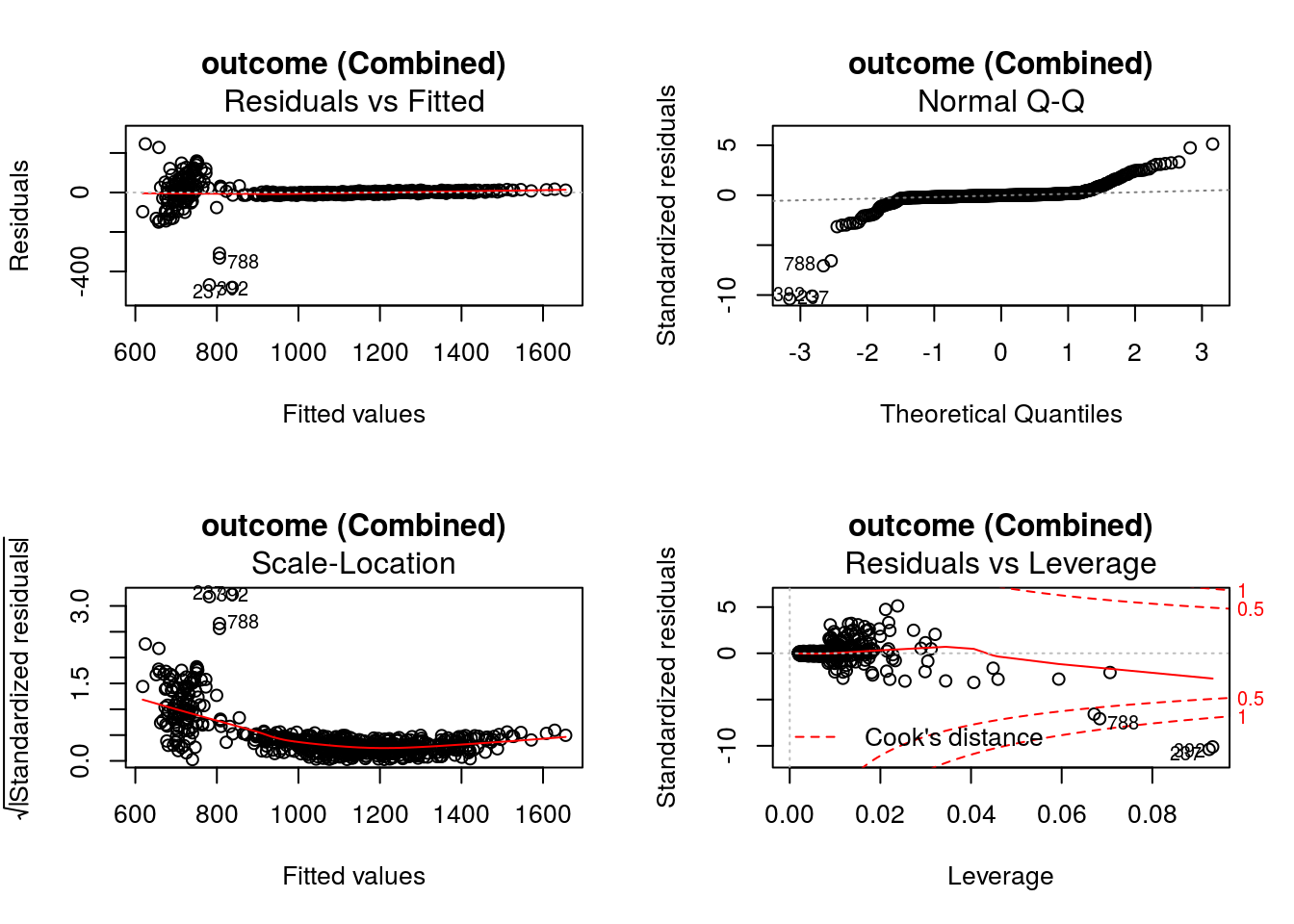
The value of input variable suppress determines of the plot titles are concatenated with an identifier of the regression analysis being plotted. For example, below we plot the Residuals vs Fitted for the outcome regression with and without the title concatenation.
graphics::par(mfrow = c(1,2))
DynTxRegime::plot(x = result2, which = 1)
DynTxRegime::plot(x = result2, suppress = TRUE, which = 1)
If there are additional diagnostic tools defined for a regression method used in the analysis but not implemented in DynTxRegime, the value object returned by the regression method can be extracted using function DynTxRegime::
fitObj <- DynTxRegime::fitObject(object = result2)
fitObj$outcome
$outcome$Combined
Call:
lm(formula = YinternalY ~ CD4_0 + CD4_6 + A2 + CD4_6:A2, data = data)
Coefficients:
(Intercept) CD4_0 CD4_6 A2 CD4_6:A2
344.9733 1.8566 -0.1238 500.7085 -1.6028 As for DynTxRegime::
is(object = fitObj$outcome$Combined)[1] "lm" "oldClass"As such, these objects can be passed to any tool defined for these classes. For example, the methods available for the object returned by the propensity regression are
utils::methods(class = is(object = fitObj$outcome$Combined)[1L]) [1] add1 alias anova case.names coerce confint cooks.distance deviance dfbeta dfbetas drop1
[12] dummy.coef effects extractAIC family formula hatvalues influence initialize kappa labels logLik
[23] model.frame model.matrix nobs plot predict print proj qr residuals rstandard rstudent
[34] show simulate slotsFromS3 summary variable.names vcov
see '?methods' for accessing help and source codeSo, to plot the residuals
graphics::plot(x = residuals(object = fitObj$outcome$Combined))
Or, to retrieve the variance-covariance matrix of the parameters
stats::vcov(object = fitObj$outcome$Combined) (Intercept) CD4_0 CD4_6 A2 CD4_6:A2
(Intercept) 123.82591625 -0.183306668 -0.0522510881 -123.0125297 0.1975916157
CD4_0 -0.18330667 0.080630743 -0.0641290567 -0.1744761 0.0001984050
CD4_6 -0.05225109 -0.064129057 0.0513346478 0.3368109 -0.0004878835
A2 -123.01252973 -0.174476057 0.3368108950 494.3847061 -0.8583301249
CD4_6:A2 0.19759162 0.000198405 -0.0004878835 -0.8583301 0.0015724341The method DynTxRegime::
DynTxRegime::outcome(object = result2)$Combined
Call:
lm(formula = YinternalY ~ CD4_0 + CD4_6 + A2 + CD4_6:A2, data = data)
Coefficients:
(Intercept) CD4_0 CD4_6 A2 CD4_6:A2
344.9733 1.8566 -0.1238 500.7085 -1.6028 Once satisfied that the postulated model is suitable, the estimated optimal treatment, the estimated \(Q\)-functions, and the estimated value for the dataset used for the analysis can be retrieved.
Function DynTxRegime::
DynTxRegime::optTx(x = result3)$optimalTx
[1] 1 0 0 1 0 0 1 0 1 0 0 1 1 0 0 1 0 1 1 0 1 1 1 0 0 0 0 0 0 1 0 0 0 0 1 1 1 1 1 0 0 1 0 1 1 1 0 1 0 0 1 1 1 0 1 1 0 1 0 1 1 0 0 0 0 1 0 0 0 0 0 1 1 0 0 1 1 1 1 0 0 0 1 0 0 0
[87] 0 0 1 1 1 1 0 0 1 0 1 1 0 0 0 1 1 1 0 1 0 0 1 1 1 0 0 0 0 1 1 0 0 0 1 0 0 1 0 1 1 1 1 1 0 1 1 0 1 1 0 1 0 0 0 0 0 0 0 0 0 1 1 1 0 1 0 1 0 1 0 0 1 1 1 0 1 0 0 0 0 1 1 0 0 0
[173] 1 1 0 0 0 0 0 0 1 0 1 1 0 1 0 0 0 1 1 1 1 1 0 0 0 0 0 1 0 0 0 0 0 1 0 0 1 1 1 0 0 1 1 0 1 0 0 1 0 1 0 0 0 0 0 1 0 1 1 0 1 1 0 1 1 0 1 1 0 1 0 0 0 0 0 1 1 0 0 0 0 0 0 1 0 1
[259] 1 0 0 1 0 1 1 0 1 1 1 0 1 0 0 0 0 1 0 0 1 1 0 0 1 1 0 0 0 0 1 0 1 1 1 1 1 0 1 1 1 1 1 0 0 0 0 1 0 0 1 0 1 0 1 0 0 0 0 0 1 1 1 0 0 1 1 1 0 1 0 0 0 1 0 1 1 0 1 1 0 0 0 0 0 0
[345] 1 1 0 1 1 0 1 0 1 0 1 0 0 0 0 0 0 1 1 0 0 1 0 0 0 1 1 1 1 1 1 0 1 0 1 1 1 1 0 0 0 0 0 0 1 0 0 1 0 0 1 1 1 0 1 0 1 1 1 0 1 1 0 1 1 1 0 1 1 1 1 1 0 1 1 1 1 1 1 0 0 1 0 0 0 1
[431] 1 1 1 0 1 1 0 0 0 0 1 0 1 1 1 0 0 1 0 0 0 1 0 1 1 1 1 1 1 0 1 1 1 0 1 1 1 1 1 1 0 0 0 1 0 1 1 1 0 1 0 0 1 0 1 0 1 1 0 0 1 1 0 1 1 1 0 0 0 0 1 1 0 0 0 0 1 0 1 1 1 0 0 0 1 0
[517] 1 1 0 0 0 1 1 0 1 0 1 0 1 1 0 0 1 0 0 1 0 0 1 0 0 0 1 0 1 0 1 0 1 0 1 0 1 1 1 0 1 1 0 0 0 1 1 1 0 1 1 0 1 1 1 1 1 0 0 1 1 1 1 1 1 0 0 0 0 0 1 0 0 1 0 0 1 1 1 1 0 0 1 1 1 1
[603] 1 1 1 1 0 0 0 0 0 0 1 1 1 0 0 0 0 0 0 1 0 1 0 1 1 0 0 1 0 0 1 0 1 1 0 0 0 1 0 1 0 1 0 1 1 0 1 0 1 0 1 0 1 1 0 0 1 0 0 0 1 0 1 0 1 1 0 1 1 1 0 1 0 0 0 1 1 1 0 1 1 1 0 1 0 1
[689] 0 1 0 0 1 0 0 1 0 1 0 1 0 0 0 1 1 1 0 1 1 0 0 0 1 0 0 1 1 1 0 0 1 0 0 1 0 1 1 0 0 0 1 0 1 0 0 1 1 1 1 0 0 0 0 1 1 1 0 1 0 0 0 0 1 0 1 1 1 1 0 1 0 1 1 0 1 0 0 1 1 0 0 1 0 0
[775] 1 1 1 1 0 1 0 1 1 0 1 0 0 1 1 0 0 1 0 1 0 1 0 0 1 0 1 1 0 0 1 1 1 1 1 1 1 0 0 1 1 1 0 1 1 1 1 1 0 1 0 0 1 1 1 0 0 0 1 1 0 0 1 1 1 1 1 0 0 0 1 1 0 1 0 1 0 1 1 0 1 1 0 1 1 1
[861] 1 0 1 0 1 0 1 0 1 0 0 0 1 1 1 0 0 0 0 0 0 0 1 0 1 0 1 1 0 0 0 1 1 1 1 1 0 0 0 1 1 1 1 0 1 0 0 1 0 0 0 1 1 1 0 1 0 1 1 1 1 0 0 0 1 0 0 0 1 1 1 0 0 0 0 0 0 0 1 0 0 1 0 1 1 0
[947] 0 1 1 0 1 1 1 0 0 1 1 1 1 1 0 1 0 0 1 1 1 0 0 0 1 1 0 0 0 0 0 1 0 0 0 0 0 1 0 0 0 0 1 1 0 1 1 1 1 1 1 0 1 1
$decisionFunc
0 1
[1,] NA NA
[2,] 1160.5977 842.6886
[3,] 1295.5570 784.5864
[4,] NA NA
[5,] 1179.9419 794.5662
[6,] 1192.1390 786.0266
[7,] NA NA
[8,] 1014.2487 851.9381
[9,] NA NA
[10,] 957.0860 873.3299
[11,] 1025.3477 840.1231
[12,] NA NA
[13,] NA NA
[14,] 1121.5400 828.1510
[15,] 1276.1801 796.7343
[16,] NA NA
[17,] 1013.9647 795.2918
[18,] NA NA
[19,] NA NA
[20,] 1534.9586 790.5978
[21,] NA NA
[22,] NA NA
[23,] NA NA
[24,] 1186.9062 798.1731
[25,] 985.8382 832.2757
[26,] 851.2325 842.8574
[27,] 1214.2343 838.2818
[28,] 939.6058 910.6080
[29,] 1107.4303 827.6893
[30,] NA NA
[31,] 1295.4751 764.6553
[32,] 1017.1256 788.1987
[33,] 988.5404 866.1410
[34,] 1020.1001 826.2648
[35,] NA NA
[36,] NA NA
[37,] NA NA
[38,] NA NA
[39,] NA NA
[40,] 1020.9274 805.8740
[41,] 1362.8748 793.3137
[42,] NA NA
[43,] 963.0181 864.5634
[44,] NA NA
[45,] NA NA
[46,] NA NA
[47,] 914.5524 856.6506
[48,] NA NA
[49,] 1021.5105 865.9389
[50,] 1024.6679 860.1806
[51,] NA NA
[52,] NA NA
[53,] NA NA
[54,] 930.6608 853.1449
[55,] NA NA
[56,] NA NA
[57,] 1404.2700 833.8452
[58,] NA NA
[59,] 1385.0927 752.3419
[60,] NA NA
[61,] NA NA
[62,] 1560.2418 794.0597
[63,] 1103.7074 836.1794
[64,] 993.1753 854.5455
[65,] 1114.4381 873.8606
[66,] NA NA
[67,] 901.2354 805.2749
[68,] 1348.6302 796.3561
[69,] 1337.9181 764.2975
[70,] 1167.0450 813.6997
[71,] 1105.9819 803.0857
[72,] NA NA
[73,] NA NA
[74,] 1214.1509 768.6579
[75,] 1473.7328 788.3458
[76,] NA NA
[77,] NA NA
[78,] NA NA
[79,] NA NA
[80,] 1053.6582 836.1380
[81,] 1073.8607 807.5800
[82,] 1080.4033 839.1259
[83,] NA NA
[84,] 1080.7252 847.4154
[85,] 1255.4377 792.9928
[86,] 1224.7488 772.6290
[87,] 1205.0975 806.9358
[88,] 1043.5020 870.6541
[89,] NA NA
[90,] NA NA
[91,] NA NA
[92,] NA NA
[93,] 1400.5933 743.5786
[94,] 1283.3381 789.7775
[95,] NA NA
[96,] 1174.5749 838.5506
[97,] NA NA
[98,] NA NA
[99,] 1278.1525 792.6947
[100,] 1478.9756 769.6179
[101,] 1179.1259 804.0849
[102,] NA NA
[103,] NA NA
[104,] NA NA
[105,] 966.2981 860.3672
[106,] NA NA
[107,] 949.4987 831.7337
[108,] 1140.0031 838.5901
[109,] NA NA
[110,] NA NA
[111,] NA NA
[112,] 993.4471 832.4832
[113,] 911.6007 832.1164
[114,] 1259.2108 819.3209
[115,] 1103.3065 776.1555
[116,] NA NA
[117,] NA NA
[118,] 1132.3853 783.4729
[119,] 1229.6209 827.6693
[120,] 1109.6465 857.0805
[121,] NA NA
[122,] 966.6728 808.4619
[123,] 1468.8839 771.6080
[124,] NA NA
[125,] 1422.3777 744.2745
[126,] NA NA
[127,] NA NA
[128,] NA NA
[129,] NA NA
[130,] NA NA
[131,] 1288.2583 819.9169
[132,] NA NA
[133,] NA NA
[134,] 1225.6128 817.7347
[135,] 815.7143 853.0842
[136,] NA NA
[137,] 1050.2364 813.5606
[138,] NA NA
[139,] 1274.6079 824.4977
[140,] 1002.7472 860.3577
[141,] 1051.0566 837.2755
[142,] 1352.6389 785.7954
[143,] 1218.3495 799.4147
[144,] 1086.1793 814.0426
[145,] 1190.2897 761.1705
[146,] 1174.7281 785.7940
[147,] 1393.8345 740.3862
[148,] NA NA
[149,] NA NA
[150,] NA NA
[151,] 1040.2836 823.3302
[152,] NA NA
[153,] 1393.2365 770.7093
[154,] NA NA
[155,] 1131.3325 829.0683
[156,] NA NA
[157,] 1064.7371 820.0303
[158,] 922.8952 852.9806
[159,] NA NA
[160,] NA NA
[161,] NA NA
[162,] 1064.2611 834.8568
[163,] NA NA
[164,] 1072.2446 805.7756
[165,] 1182.2829 828.0866
[166,] 1222.9475 843.7485
[167,] 1401.1909 779.3902
[168,] NA NA
[169,] NA NA
[170,] 1358.9102 751.4806
[171,] 1412.1166 812.5362
[172,] 1114.6502 809.2403
[173,] NA NA
[174,] NA NA
[175,] 1358.1822 798.4044
[176,] 960.5003 839.8363
[177,] 913.5732 867.9974
[178,] 1645.5201 767.9744
[179,] 1145.8626 799.2277
[180,] 1093.1822 766.3412
[181,] NA NA
[182,] 1086.6037 804.0528
[183,] NA NA
[184,] NA NA
[185,] 1269.3268 806.8053
[186,] NA NA
[187,] 1312.6255 793.1363
[188,] 1013.8961 812.8280
[189,] 1225.0993 768.2643
[190,] NA NA
[191,] NA NA
[192,] 603.8915 870.3781
[193,] NA NA
[194,] NA NA
[195,] 1491.1023 787.7269
[196,] 1191.5523 787.0966
[197,] 1214.0711 794.5509
[198,] 931.4038 802.6140
[199,] 1140.9241 848.9239
[200,] NA NA
[201,] 1196.3323 829.4463
[202,] 1231.9135 806.9676
[203,] 1140.1203 815.3723
[204,] 1230.8715 809.4177
[205,] 1155.1878 765.8431
[206,] NA NA
[207,] 1433.0773 785.2315
[208,] 1297.8368 760.8431
[209,] NA NA
[210,] NA NA
[211,] NA NA
[212,] 1033.4850 799.6344
[213,] 1376.3121 829.1545
[214,] NA NA
[215,] NA NA
[216,] 1179.8659 798.4574
[217,] NA NA
[218,] 999.3412 820.1606
[219,] 1048.1102 791.5444
[220,] NA NA
[221,] 1268.3736 811.0759
[222,] NA NA
[223,] 1505.0641 753.3637
[224,] 1316.8417 811.0544
[225,] 1162.0953 838.0613
[226,] 994.5937 858.1567
[227,] 1622.0372 767.0732
[228,] NA NA
[229,] 991.7268 867.3392
[230,] NA NA
[231,] NA NA
[232,] 1064.6330 860.2447
[233,] NA NA
[234,] NA NA
[235,] 1165.5376 822.4149
[236,] NA NA
[237,] NA NA
[238,] 1055.5046 773.8871
[239,] NA NA
[240,] NA NA
[241,] 1113.7754 784.8601
[242,] NA NA
[243,] 912.1939 832.9679
[244,] 1229.1983 780.2374
[245,] 1232.7112 800.7001
[246,] 1153.5700 827.7265
[247,] 1340.5247 751.3363
[248,] NA NA
[249,] NA NA
[250,] 1149.4384 773.6055
[251,] 1178.1614 766.5474
[252,] 1298.0896 818.9403
[253,] 1195.3902 858.3219
[254,] 1223.2376 802.9193
[255,] 906.7935 831.2324
[256,] NA NA
[257,] 1363.9555 766.2689
[258,] NA NA
[259,] NA NA
[260,] 1178.3491 810.3167
[261,] 1274.2290 765.8897
[262,] NA NA
[263,] 1136.2824 810.3523
[264,] 793.4483 831.6811
[265,] NA NA
[266,] 980.9688 775.0797
[267,] NA NA
[268,] 909.6437 912.2015
[269,] NA NA
[270,] 1226.5484 811.4343
[271,] NA NA
[272,] 1421.2288 739.6441
[273,] 1218.9626 765.2073
[274,] 1271.6138 779.1345
[275,] 1468.2739 772.0368
[276,] NA NA
[277,] 1252.0514 815.0682
[278,] 1281.6850 796.3638
[279,] NA NA
[280,] NA NA
[281,] 927.4769 831.2453
[282,] 1188.4655 796.9533
[283,] NA NA
[284,] NA NA
[285,] 962.5292 823.3606
[286,] 1162.0883 801.1151
[287,] 958.1313 839.3497
[288,] 1068.1885 840.0516
[289,] NA NA
[290,] 1131.5595 821.1821
[291,] NA NA
[292,] NA NA
[293,] 794.3360 838.6133
[294,] NA NA
[295,] NA NA
[296,] 1419.3288 735.2356
[297,] NA NA
[298,] NA NA
[299,] NA NA
[300,] NA NA
[301,] NA NA
[302,] 939.6053 839.8927
[303,] 1080.8015 854.3201
[304,] 1286.0417 801.7070
[305,] 1105.6447 783.1799
[306,] NA NA
[307,] 1026.2831 877.7499
[308,] 1390.5120 781.3852
[309,] NA NA
[310,] 1250.0856 851.2919
[311,] NA NA
[312,] 1179.7362 783.4426
[313,] NA NA
[314,] 1098.6886 813.0397
[315,] 1015.4921 784.1749
[316,] 1323.8446 789.9592
[317,] 1085.6601 846.7638
[318,] 1382.2822 797.5876
[319,] NA NA
[320,] NA NA
[321,] NA NA
[322,] 1113.8141 837.6425
[323,] 1024.5780 869.6637
[324,] NA NA
[325,] NA NA
[326,] NA NA
[327,] 1286.7678 727.2216
[328,] NA NA
[329,] 1311.4563 824.9714
[330,] 994.4049 830.4222
[331,] 1155.8538 793.1750
[332,] NA NA
[333,] 1014.8862 826.7715
[334,] NA NA
[335,] NA NA
[336,] 904.9082 820.1249
[337,] NA NA
[338,] NA NA
[339,] 1067.7542 806.4813
[340,] 963.2655 835.6367
[341,] 1093.3112 796.0396
[342,] 1164.5872 808.9816
[343,] 1282.6672 843.7258
[344,] 1312.7521 816.0309
[345,] NA NA
[346,] NA NA
[347,] 978.8905 867.2902
[348,] NA NA
[349,] NA NA
[350,] 1009.5239 781.2358
[351,] 694.6397 835.4257
[352,] 1203.2341 788.0360
[353,] NA NA
[354,] 1065.8894 804.6128
[355,] 825.0359 825.7886
[356,] 1203.9186 809.7554
[357,] 1444.1601 800.8614
[358,] 954.9516 849.1462
[359,] 1083.7103 800.2766
[360,] 1452.9010 789.6399
[361,] 1269.7265 790.2539
[362,] NA NA
[363,] NA NA
[364,] 1076.2409 790.4612
[365,] 1014.4196 801.6635
[366,] NA NA
[367,] 885.6018 864.8292
[368,] 1160.8898 809.1301
[369,] 1097.2397 808.6842
[370,] NA NA
[371,] NA NA
[372,] NA NA
[373,] NA NA
[374,] NA NA
[375,] NA NA
[376,] 1129.8416 803.2188
[377,] NA NA
[378,] 986.9374 825.5797
[379,] NA NA
[380,] NA NA
[381,] NA NA
[382,] NA NA
[383,] 1004.7020 819.9767
[384,] 1358.7406 755.0171
[385,] 1254.8339 799.3446
[386,] 1318.8515 781.1508
[387,] 1283.2391 813.6844
[388,] 1164.0680 815.8061
[389,] 848.8770 888.6578
[390,] 1147.6720 832.9081
[391,] 1390.6168 802.9971
[392,] NA NA
[393,] 972.6987 861.3829
[394,] 1304.7880 812.8125
[395,] NA NA
[396,] NA NA
[397,] NA NA
[398,] 1196.4081 763.7308
[399,] NA NA
[400,] 939.5323 801.0834
[401,] NA NA
[402,] NA NA
[403,] NA NA
[404,] 950.4036 844.2949
[405,] NA NA
[406,] NA NA
[407,] 1362.1317 769.7825
[408,] NA NA
[409,] NA NA
[410,] NA NA
[411,] 856.5621 823.9932
[412,] NA NA
[413,] NA NA
[414,] NA NA
[415,] NA NA
[416,] NA NA
[417,] 1311.7432 825.8269
[418,] NA NA
[419,] NA NA
[420,] NA NA
[421,] NA NA
[422,] NA NA
[423,] NA NA
[424,] 1136.5338 812.6684
[425,] 1231.6474 849.8722
[426,] NA NA
[427,] 1383.2482 767.1623
[428,] 1123.4232 784.5950
[429,] 885.8766 834.7193
[430,] NA NA
[431,] NA NA
[432,] NA NA
[433,] NA NA
[434,] 976.5020 840.2754
[435,] NA NA
[436,] NA NA
[437,] 1394.8683 779.8697
[438,] 1232.6794 786.0314
[439,] 882.6742 843.4883
[440,] 1112.3779 824.8084
[441,] NA NA
[442,] 1082.7687 820.7832
[443,] NA NA
[444,] NA NA
[445,] NA NA
[446,] 1350.4229 765.5989
[447,] 1155.4964 821.5593
[448,] NA NA
[449,] 1166.7167 823.6101
[450,] 1468.6653 760.4771
[451,] 1171.3326 822.1925
[452,] NA NA
[453,] 1344.2934 766.4252
[454,] NA NA
[455,] NA NA
[456,] NA NA
[457,] NA NA
[458,] NA NA
[459,] NA NA
[460,] 1420.4094 761.9286
[461,] NA NA
[462,] NA NA
[463,] NA NA
[464,] 1232.7906 815.6250
[465,] NA NA
[466,] NA NA
[467,] NA NA
[468,] NA NA
[469,] NA NA
[470,] NA NA
[471,] 1362.9130 831.8398
[472,] 1268.2831 833.2905
[473,] 1147.6349 759.5028
[474,] NA NA
[475,] 1101.6042 831.0019
[476,] NA NA
[477,] NA NA
[478,] NA NA
[479,] 1300.3866 794.0112
[480,] NA NA
[481,] 970.4243 802.1543
[482,] 1316.5399 778.9818
[483,] 806.7189 829.2926
[484,] 1178.7277 792.7320
[485,] NA NA
[486,] 1667.2267 742.0177
[487,] NA NA
[488,] NA NA
[489,] 1221.1338 773.6295
[490,] 1397.3492 751.4952
[491,] NA NA
[492,] NA NA
[493,] 1504.6957 790.3405
[494,] NA NA
[495,] NA NA
[496,] NA NA
[497,] 1490.8591 721.2443
[498,] 1193.9784 792.7224
[499,] 1235.2840 806.1447
[500,] 1415.9835 812.5152
[ reached getOption("max.print") -- omitted 500 rows ]The object returned is a list. The element names are $optimalTx and $decisionFunc, corresponding to the \(\widehat{d}^{opt}_{Q,k}(H_{ki}; \widehat{\beta}_{k})\) and the estimated \(Q\)-functions at each treatment option, respectively.
When provided the value object returned by the final step of the Q-learning algorithm, function DynTxRegime::
DynTxRegime::estimator(x = result1)[1] 1112.179Function DynTxRegime::
The first new patient has the following baseline covariates
print(x = patient1) CD4_0
1 457The recommended treatment based on the previous first stage analysis is obtained by providing the object returned by qLearn() as well as a data.frame object that contains the baseline covariates of the new patient.
DynTxRegime::optTx(x = result1, newdata = patient1)$optimalTx
[1] 0
$decisionFunc
0 1
[1,] 1125.578 720.3918Treatment A1= 0 is recommended.
Assume that patient1 receives the recommended first stage treatment, and \(x_{2}\) is measured six months after treatment. The available history is now
print(x = patient1) CD4_0 A1 CD4_6
1 457 0 576.9The recommended treatment based on the previous second stage analysis is obtained by providing the object returned by qLearn() as well as a data.frame object that contains the available covariates and treatment history of the new patient.
DynTxRegime::optTx(x = result2, newdata = patient1)$optimalTx
[1] 0
$decisionFunc
0 1
[1,] 1121.99 698.0497Treatment A2= 0 is recommended.
Again, patient1 receives the recommended treatment, and \(x_{3}\) is measured six months after treatment. The available history is now
print(x = patient1) CD4_0 A1 CD4_6 A2 CD4_12
1 457 0 576.9 0 460.6Finally recommended treatment based on the previous third stage analysis is obtained by providing the object returned by qLearn() as well as a data.frame object that contains the available covariates and treatment history of the new patient.
DynTxRegime::optTx(x = result3, newdata = patient1)$optimalTx
[1] 0
$decisionFunc
0 1
[1,] 1119.145 810.0593Treatment A3= 0 is recommended.
Note that though the estimated optimal treatment regime was obtained starting at stage \(K\) and ending at stage 1, predicted optimal treatment regimes for new patients clearly must be obtained starting at the first stage. Predictions for subsequent stages cannot be obtained until the mid-stage covariate information becomes available.
Value Search Estimators
The augmented inverse probability weighted estimator for \(\mathcal{V}(d_{\eta})\) for fixed \(\eta\) is
\[ \begin{align} \widehat{\mathcal{V}}_{AIPW}(d_{\eta}) = n^{-1} \sum_{i=1}^{n} \left[ \frac{\mathcal{C}_{d_{\eta},i} Y_{i}} {\left\{\prod_{k=2}^{K} \pi_{d_{\eta,k}}(\overline{X}_{ki}; \overline{\eta}_{k}, \widehat{\gamma}_{k})\right\}\pi_{d_{\eta,1}}(X_{1i}; \eta_{1}, \widehat{\gamma}_{1})} \\ + \sum_{k=1}^K \left\{ \frac{\mathcal{C}_{\overline{d}_{\eta},k-1,i}}{\overline{\pi}_{d_{\eta},k-1}(\overline{X}_{k-1,i}; \widehat{\overline{\gamma}}_{k-1})} - \frac{\mathcal{C}_{\overline{d}_{\eta},k,i}}{\overline{\pi}_{d_{\eta},k}(\overline{X}_{ki}; \widehat{\overline{\gamma}}_{k})}\right\} \mathcal{Q}_{d_{\eta},k}(\overline{X}_{ki};\widehat{\beta}_{k}) \right], \end{align} \]
where \(C_{d_{\eta}} = \text{I}\{\overline{A} = \overline{d}_{\eta}(\overline{X})\}\);
\[ \pi_{d_{\eta,1}}(X_{1};\gamma_{1}) = \omega_{1}(X_{1},1;\gamma_{1})\text{I}\{d_{\eta,1}(X_{1}) = 1\} + \omega_{1}(X_{1},0;\gamma_{1})\text{I}\{d_{\eta,1}(X_{1}) = 0\}, \]
\[ \begin{align} \pi_{d_{\eta,k}}(\overline{X}_{k};\gamma_{k}) =& \omega_{k}\{\overline{X}_{k}, \overline{d}_{\eta,k-1}(\overline{X}_{k-1}),1;\gamma_{k}\} ~ ~ \text{I}[d_{\eta,k}\{\overline{X}_{k},\overline{d}_{\eta,k-1}(\overline{X}_{k-1})\} = 1] \\ &+ \omega_{k}\{\overline{X}_{k}, \overline{d}_{\eta,k-1}(\overline{X}_{k-1}),0;\gamma_{k}\}~~\text{I}[d_{\eta,k}\{\overline{X}_{k},\overline{d}_{\eta,k-1}(\overline{X}_{k-1})\} = 0]. \end{align} \]
Further \(\omega_{k}(h_{k},a_{k};\gamma_{k})\), \(k = 1, \dots, K\) are models for the propensity scores \(P(A_{k} = a_{k}| H_{k} = h_{k})\), and \(\widehat{\gamma}_{k}\) is a suitable estimator for \(\gamma_{k}\), \(k = 1, \dots, K\).
Finally, \(\mathcal{Q}_{d_{\eta},k}(\overline{X}_{ki};\widehat{\beta}_{k})\) are models for the conditional expectations \(E\{Y^{\text{*}}(d_{\eta})|\overline{X}^{\text{*}}_{k}(\overline{d}_{\eta,k-1}) = \overline{x}_{k}\}, k = 1, \dots, K\). The IPW estimator is the special case of setting these to zero.
We follow the strategy advocated in the original manuscript to estimate \(\mathcal{Q}_{d_{\eta},k}(\overline{X}_{ki};\widehat{\beta}_{k})\). That is, we posit model \(Q_{k}(h_{k}, a_{k}; \beta_{k})\) for the Q-function \(Q_{k}(h_{k},a_{k}), k = 1, \dots K\) and carry out Q-learning to obtain \(\widehat{\beta}_{k}\) and then take
\[ \mathcal{Q}_{d_{\eta},k}(\overline{X}_{ki};\widehat{\beta}_{k}) = Q_{k}\{\overline{X}_{ki}, \overline{d}_{\eta,k}(\overline{X}_{ki}); \widehat{\beta}_{k}\}, \quad k = 1, \dots K. \]
Substituting this into the value expression, the optimal treatment regime, \(\widehat{d}_{\eta,AIPW}^{opt} = \{d_{1}(h_{1},\widehat{\eta}_{1,AIPW}^{opt}), \dots, d_{K}(h_{K},\widehat{\eta}_{K,AIPW}^{opt})\}\), is obtained by maximizing \(\widehat{\mathcal{V}}_{AIPW}(d_{\eta})\) in \(\eta = (\eta_{1}, \dots, \eta_{K})\).
A general implementation of the value search estimator is provided in
The function call for DynTxRegime::
utils::str(object = DynTxRegime::optimalSeq)function (..., moPropen, moMain, moCont, data, response, txName, regimes, fSet = NULL, refit = FALSE, iter = 0L, verbose = TRUE) We briefly describe the input arguments for DynTxRegime::
| Input Argument | Description |
|---|---|
| \(\dots\) | Additional inputs to be provided to genetic algorithm. See below for additional details. |
| moPropen | A list of “modelObj” objects. The modeling objects for the \(K\) propensity regression steps. |
| moMain | A list of “modelObj” objects. The modeling objects for the \(\nu_{k}(h_{k}, a_{k}; \phi_{k})\) component of \(Q_{k}(h_{k},a_{k};\beta_{k})\) for \(k = 1, K\). Not used for IPW estimator. |
| moCont | A list of “modelObj” objects. The modeling object for the \(\text{C}_{k}(h_{k}, a_{k}; \psi_{k})\) component of \(Q_{k}(h_{k},a_{k};\beta_{k})\) for \(k = 1, K\). Not used for IPW estimator. |
| data | A “data.frame” object. The covariate history and the treatments received. |
| response | A “numeric” vector. The outcome of interest, where larger values are better. |
| txName | A “character” “vector” object. The column headers of data corresponding to the treatment variables. The ordering should coincide with the stage, i.e., the \(k^{th}\) element contains the \(k^{th}\) stage treatment. |
| regimes | A list of “function” objects. Each element of the list is a user defined function specifying the class of treatment regime under consideration. The ordering should coincide with the stage, i.e., the \(k^{th}\) element contains the \(k^{th}\) stage regime. |
| fSet | A list of “function” objects. Each element of the list is a user defined function specifying treatment or model subset structure for the decision point. The ordering should coincide with the stage, i.e., the \(k^{th}\) element contains the \(k^{th}\) stage treatment or model subset structure. |
| refit | Deprecated. |
| iter | An “integer” object. The maximum number of iterations for iterative algorithm. |
| verbose | A “logical” object. If TRUE progress information is printed to screen. |
Methods implemented in DynTxRegime break the Q-function model into two components: a main effects component and a contrasts component. For example, for binary treatments, \(Q_{k}(h_{k}, a_{k}; \beta_{k})\) can be written as
\[ Q_{k}(h_{k}, a_{k}; \beta_{k})= \nu_{k}(h_{k}; \phi_{k}) + a_{k} \text{C}_{k}(h_{k}; \psi_{k}), \text{for} ~ k = 1, \dots, K \]
where \(\beta_{k} = (\phi^{\intercal}_{k}, \psi^{\intercal}_{k})^{\intercal}\). Here, \(\nu_{k}(h_{k}; \phi_{k})\) comprises the terms of the model that are independent of treatment (so called “main effects” or “common effects”), and \(\text{C}_{k}(h_{k}; \psi_{k})\) comprises the terms of the model that interact with treatment (so called “contrasts”). Input arguments moMain and moCont specify \(\nu_{k}(h_{k}; \phi_{k})\) and \(\text{C}_{k}(h_{k}; \psi_{k})\), respectively.
In the examples provided in this chapter, the two components of each \(Q_{k}(h_{k}, a_{k}; \beta_{k})\) are both linear models, the parameters of which are estimated using stats::
Input fSet is a list of length \(K\) containing the user-defined functions specifying the feasible sets at each decision point. The only requirements for these functions are:
- The formal input argument(s) of each function must be either data or the individual covariates required for identifying subset membership.
- Each function must return a list containing two elements $subsets and $txOpts.
Element $subsets of the returned list is itself a list; each element of the list contains a nickname and the treatment options for a single feasible set.
Element $txOpts of the returned list is a character vector providing the nickname of the feasible set to which each individual is assigned. - There are no requirements for the function names or the structure of the functions’ contents.
See the Analysis tab for explicit examples.
The value object returned by DynTxRegime::
| Slot Name | Description |
|---|---|
| @analysis@genetic | The genetic algorithm results. |
| @analysis@propen | The propensity regression analysis. |
| @analysis@outcome | The outcome regression analysis. NA if IPW. |
| @analysis@regime | The \(\widehat{d}^{opt}_{\eta}\) definition. |
| @analysis@call | The unevaluated function call. |
| @analysis@optimal | The estimated value and optimal treatment for the training data. |
There are several methods available for objects of this class that assist with model diagnostics, the exploration of training set results, and the estimation of optimal treatments for future patients. We explore some of these methods under the Methods tab.
Because no Q-functions are modeled for the IPW estimator, moMain and moCont are not provided as input or are set to NULL and iter is 0 (its default value).
Input moPropen is a list of modeling objects for the propensity score regressions. In our example, the \(k^{th}\) element of the list corresponds to the modeling object for the propensity score model for \(\omega_{k}(h_k,a_{k}) = P(A_{k}=a_{k}|H_{k} = h_{k})\). Specifically, the propensity score models for each decision point are
\[ \text{logit}\left\{\omega_{1}(h_{1},1;\gamma_{1})\right\} = \gamma_{10} + \gamma_{11}~\text{CD4_0}, \]
\[ \text{logit}\left\{\omega_{2,2}(h_{2},1;\gamma_{2})\right\} = \gamma_{20} + \gamma_{21}~\text{CD4_6}, \]
and
\[ \text{logit}\left\{\omega_{3,2}(h_{3},1;\gamma_{3})\right\} = \gamma_{30} + \gamma_{31}~\text{CD4_12}, \]
where \(\text{logit}(p) = \text{log} \{p/(1-p)\}\). The modeling objects for these models are as follows
p1 <- modelObj::buildModelObj(model = ~ CD4_0,
solver.method = 'glm',
solver.args = list(family='binomial'),
predict.method = 'predict.glm',
predict.args = list(type='response'))p2 <- modelObj::buildModelObj(model = ~ CD4_6,
solver.method = 'glm',
solver.args = list(family='binomial'),
predict.method = 'predict.glm',
predict.args = list(type='response'))and
p3 <- modelObj::buildModelObj(model = ~ CD4_12,
solver.method = 'glm',
solver.args = list(family='binomial'),
predict.method = 'predict.glm',
predict.args = list(type='response'))To see a brief synopsis of the model diagnostics for these models, see header \(\omega_{k}(h_{k},a_{k};\gamma_{k})\) in the sidebar menu.
As for all methods discussed in this chapter: the “data.frame” containing all covariates and treatments received is data set dataMDPF, the treatments are contained in columns $A1, $A2, and $A3 of dataMDPF, and the response is $Y of dataMDPF.
To allow for direct comparison with the other estimators discussed in this chapter, the restricted classes of regimes that we will consider are characterized by rules of the form
\[ \begin{align} d_{\eta} &= \{d_{1}(h_{1};\eta_{1}), d_{2}(h_{2};\eta_{2}), d_{3}(h_{3};\eta_{3})\} \\ d_{1}(h_{1};\eta_{1}) &= \text{I}(\text{CD4_0} < \eta_{1}) \\ d_{2}(h_{2};\eta_{2}) &= a_{1} + (1-a_{1})~\text{I}(\text{CD4_6} < \eta_{2}) \\ d_{3}(h_{3};\eta_{3}) &= a_{2} + (1-a_{2})~\text{I}(\text{CD4_12} < \eta_{3}). \end{align} \]
The rules are specified using a list of user-defined functions, which is passed to the method through input regimes. Each user-defined function must accept as input the regime parameter name(s) and the data set, and the function must return a vector of the recommended treatment. For this example, the functions can be specified as
r1 <- function(eta1, data){ return(as.integer(x = {data$CD4_0 < eta1})) }
r2 <- function(eta2, data){ return(data$A1 + {1L-data$A1}*{data$CD4_6 < eta2}) }
r3 <- function(eta3, data){ return(data$A2 + {1L-data$A2}*{data$CD4_12 < eta3}) }
regimes <- list(r1, r2, r3)where inputs eta1, eta2, and eta3 are the parameters of the regime to be estimated and data is the same “data.frame” object passed to DynTxRegime::
- defines the regime for the entire data set, and
- returns values of the same class as the treatment variable.
- the search space for the \(\eta\) parameters,
- initial guess for the \(\eta\) parameters, and
- population size for the algorithm.
Because rgenoud::
Domains <- rbind( c(min(x = dataMDPF$CD4_0) - 0.1, max(x = dataMDPF$CD4_0) + 0.1),
c(min(x = dataMDPF$CD4_6) - 0.1, max(x = dataMDPF$CD4_6) + 0.1),
c(min(x = dataMDPF$CD4_12) - 0.1, max(x = dataMDPF$CD4_12) + 0.1))
starting.values <- c(mean(x = dataMDPF$CD4_0), mean(x = dataMDPF$CD4_6), mean(x = dataMDPF$CD4_12))
pop.size <- 1000LFor additional information on these and other available inputs for the genetic algorithm, please see ?rgenound::genoud.
Because not all treatments are available to all patients, we must define fSet, a function defining the treatment subset structure. Specifically, the feasible sets are defined to be
\[ \Psi_{1}(h_{1}) = \{0,1\}~\{s_{1}(h_{1}) = 1\} \]
\[ \Psi_{2}(h_{2}) = \left\{ \begin{array}{cl} \{1\} \subset \mathcal{A}_{2} & \text{if } A_{1} = 1 ~\{s_{2}(h_{2}) = 1\}\\ \{ 0,1\} \subset \mathcal{A}_{2}& \text{if } A_{1} = 0~\{s_{2}(h_{2}) = 2\}\\ \end{array} \right. . \]
\[ \Psi_{3}(h_{3}) = \left\{ \begin{array}{cl} \{1\} \subset \mathcal{A}_{3} & \text{if } A_{2} = 1~\{s_{3}(h_{3}) = 1\}\\ \{ 0,1\} \subset \mathcal{A}_{3}& \text{if } A_{2} = 0~\{s_{3}(h_{3}) = 2\}\\ \end{array} \right. . \]
That is, individuals that received treatment 1 remain on treatment 1 in all subsequent treatment decisions. All others are assigned one of \(\{0,1\}\). User-defined functions that defines the feasible treatments for the \(K\) decisions are
fSet1 <- function(data){
subsets <- list(list("s1",c(0L,1L)))
txOpts <- rep(x = 's1', times = nrow(x = data))
return(list("subsets" = subsets, "txOpts" = txOpts))
}fSet2 <- function(data){
subsets <- list(list("s1",1L),
list("s2",c(0L,1L)))
txOpts <- rep(x = 's2', times = nrow(x = data))
txOpts[data$A1 == 1L] <- "s1"
return(list("subsets" = subsets, "txOpts" = txOpts))
}fSet3 <- function(data){
subsets <- list(list("s1",1L),
list("s2",c(0L,1L)))
txOpts <- rep(x = 's2', times = nrow(x = data))
txOpts[data$A2 == 1L] <- "s1"
return(list("subsets" = subsets, "txOpts" = txOpts))
}fSet = list(fSet1, fSet2, fSet3)The optimal treatment regime, \(\widehat{d}_{\eta, IPW}^{opt}(h_{1})\), is estimated as follows.
IPW <- DynTxRegime::optimalSeq(moPropen = list(p1, p2, p3),
data = dataMDPF,
response = dataMDPF$Y,
txName = c('A1','A2','A3'),
fSet = fSet,
regimes = regimes,
Domains = Domains,
pop.size = pop.size,
starting.values = starting.values,
verbose = TRUE)IPW estimator will be used
Value Search - Coarsened Data Perspective 3 Decision Points
Decision point 1
Subsets of treatment identified as:
$s1
[1] 0 1
Number of patients in data for each subset:
s1
1000
Decision point 2
Subsets of treatment identified as:
$s1
[1] 1
$s2
[1] 0 1
Number of patients in data for each subset:
s1 s2
368 632
Decision point 3
Subsets of treatment identified as:
$s1
[1] 1
$s2
[1] 0 1
Number of patients in data for each subset:
s1 s2
486 514
Propensity for treatment regression.
Decision point 1
1000 included in analysis
Regression analysis for moPropen:
Call: glm(formula = YinternalY ~ CD4_0, family = "binomial", data = data)
Coefficients:
(Intercept) CD4_0
2.385956 -0.006661
Degrees of Freedom: 999 Total (i.e. Null); 998 Residual
Null Deviance: 1316
Residual Deviance: 1227 AIC: 1231
Decision point 2 subset s1 excluded from propensity regression632 included in analysis
Regression analysis for moPropen:
Call: glm(formula = YinternalY ~ CD4_6, family = "binomial", data = data)
Coefficients:
(Intercept) CD4_6
1.234491 -0.004781
Degrees of Freedom: 631 Total (i.e. Null); 630 Residual
Null Deviance: 608.5
Residual Deviance: 577.8 AIC: 581.8
Decision point 3 subset s1 excluded from propensity regression514 included in analysis
Regression analysis for moPropen:
Call: glm(formula = YinternalY ~ CD4_12, family = "binomial", data = data)
Coefficients:
(Intercept) CD4_12
0.929409 -0.003816
Degrees of Freedom: 513 Total (i.e. Null); 512 Residual
Null Deviance: 622.5
Residual Deviance: 609.1 AIC: 613.1
Outcome regression.
No outcome regression performed.
Tue Jul 21 12:16:02 2020
Domains:
1.102936e+02 <= X1 <= 7.696901e+02
1.408169e+02 <= X2 <= 9.557700e+02
8.946612e+01 <= X3 <= 7.716485e+02
Data Type: Floating Point
Operators (code number, name, population)
(1) Cloning........................... 122
(2) Uniform Mutation.................. 125
(3) Boundary Mutation................. 125
(4) Non-Uniform Mutation.............. 125
(5) Polytope Crossover................ 125
(6) Simple Crossover.................. 126
(7) Whole Non-Uniform Mutation........ 125
(8) Heuristic Crossover............... 126
(9) Local-Minimum Crossover........... 0
HARD Maximum Number of Generations: 100
Maximum Nonchanging Generations: 10
Population size : 1000
Convergence Tolerance: 1.000000e-03
Not Using the BFGS Derivative Based Optimizer on the Best Individual Each Generation.
Not Checking Gradients before Stopping.
Using Out of Bounds Individuals.
Maximization Problem.
Generation# Solution Value
0 1.163353e+03
1 1.175976e+03
2 1.183261e+03
3 1.184656e+03
8 1.188721e+03
'wait.generations' limit reached.
No significant improvement in 10 generations.
Solution Fitness Value: 1.188721e+03
Parameters at the Solution:
X[ 1] : 3.207142e+02
X[ 2] : 2.986535e+02
X[ 3] : 3.446335e+02
Solution Found Generation 8
Number of Generations Run 19
Tue Jul 21 12:24:24 2020
Total run time : 0 hours 8 minutes and 22 seconds
Genetic Algorithm
$value
[1] 1188.721
$par
[1] 320.7142 298.6535 344.6335
$gradients
[1] NA NA NA
$generations
[1] 19
$peakgeneration
[1] 8
$popsize
[1] 1000
$operators
[1] 122 125 125 125 125 126 125 126 0
$dp=1
Recommended Treatments:
0 1
918 82
$dp=2
Recommended Treatments:
0 1
918 82
$dp=3
Recommended Treatments:
0 1
852 148
Estimated Value: 1188.721 Above, we opted to set verbose to TRUE to highlight some of the information that should be verified by a user. Notice the following:
- The first line of the verbose output indicates that the selected value estimator is the IPW estimator and that the estimator is from the coarsened data perspective with 3 decision points.
Users should verify that this is the intended estimator and the correct number of decision points. - The information provided for the propensity regressions are not defined within DynTxRegime::
optimalSeq() , but are specified by the statistical method selected to obtain parameter estimates; in this example it is defined by stats::glm() .
Users should verify that the models were correctly interpreted by the software and that there are no warnings or messages reported by the regression methods. - A statement indicates that no outcome regression was performed as is expected for the IPW estimator.
- The results of the genetic algorithm used to optimize over \(\eta\) show the estimated value \(\widehat{\mathcal{V}}_{IPW}(d_{\eta})\) and the estimated parameters of the optimal restricted regime.
Users should verify that the regime was correctly interpreted by the software and that there are no warnings or messages reported by rgenoud::genoud() . - Finally, a tabled summary of the recommended treatments and the estimated value for the training data are shown.
The first step of the post-analysis should always be model diagnostics. DynTxRegime comes with several tools to assist in this task. However, we have explored the propensity score models previously and will skip that step here. Many of the model diagnostic tools are described under the Methods tab.
The estimated parameters of the optimal treatment regime can be retrieved using DynTxRegime::
DynTxRegime::regimeCoef(object = IPW)$`dp=1`
eta1
320.7142
$`dp=2`
eta2
298.6535
$`dp=3`
eta3
344.6335 From this we see that the estimated optimal treatment regime is
\[ \begin{align} d_{\eta} &= \{d_{1}(h_{1};\eta_{1}), d_{2}(h_{2};\eta_{2}), d_{3}(h_{3};\eta_{3})\} \\ d_{1}(h_{1};\eta_{1}) &= \text{I}(\text{CD4_0} < 320.71) \\ d_{2}(h_{2};\eta_{2}) &= a_{1} + (1-a_{1})~\text{I}(\text{CD4_6} < 298.65) \\ d_{3}(h_{3};\eta_{3}) &= a_{2} + (1-a{2})~\text{I}(\text{CD4_12} < 344.63). \end{align} \]
The estimated value under the optimal treatment regime for the training data can be retrieved using DynTxRegime::
DynTxRegime::estimator(x = IPW)[1] 1188.721There are several methods available for the returned object that assist with model diagnostics, the exploration of training set results, and the estimation of optimal treatments for future patients. A complete description of these methods can be found under the Methods tab.
Inputs moMain and moCont are modeling objects specifying the models posited for the \(K\) Q-functions. In our example, the \(k^{th}\) element of the list corresponds to the modeling object for the Q-function model \(Q_{k}(h_{k},a_{k})\). Specifically, the models for each decision point are
\[ Q_{1}(h_{1},a_{1};\beta_{1}) = \beta_{10} + \beta_{11} \text{CD4_0} + a_{1}~(\beta_{12} + \beta_{13} \text{CD4_0}), \]
\[ Q_{2}(h_{2},a_{2};\beta_{2}) = \beta_{20} + \beta_{21} \text{CD4_0} + \beta_{22} \text{CD4_6} + a_{2}~(\beta_{23} + \beta_{24} \text{CD4_6}), \]
and
\[ Q_{3}(h_{3},a_{3};{\beta}_{3}) = {\beta}_{30} + {\beta}_{31} \text{CD4_0} + {\beta}_{32} \text{CD4_6} + {\beta}_{33} \text{CD4_12} + a_{3}~({\beta}_{34} + {\beta}_{35} \text{CD4_12}). \]
The modeling objects for these models are as follows
q1Main <- modelObj::buildModelObj(model = ~ CD4_0,
solver.method = 'lm',
predict.method = 'predict.lm')q1Cont <- modelObj::buildModelObj(model = ~ CD4_0,
solver.method = 'lm',
predict.method = 'predict.lm')q2Main <- modelObj::buildModelObj(model = ~ CD4_0 + CD4_6,
solver.method = 'lm',
predict.method = 'predict.lm')q2Cont <- modelObj::buildModelObj(model = ~ CD4_6,
solver.method = 'lm',
predict.method = 'predict.lm')and
q3Main <- modelObj::buildModelObj(model = ~ CD4_0 + CD4_6 + CD4_12,
solver.method = 'lm',
predict.method = 'predict.lm')q3Cont <- modelObj::buildModelObj(model = ~ CD4_12,
solver.method = 'lm',
predict.method = 'predict.lm')To see a brief synopsis of the model diagnostics for these models, see header \(Q_{k}(h_{k}, a_{k};\beta_{k})\) in the sidebar menu.
Input moPropen is a list of modeling objects for the propensity score regressions. In our example, the \(k^{th}\) element of the list corresponds to the modeling object for the propensity score model for \(\omega_{k}(h_k,a_{k}) = P(A_{k}=a_{k}|H_{k} = h_{k})\). Specifically, the propensity score models for each decision point are
\[ \text{logit}\left\{\omega_{1}(h_{1},1;\gamma_{1})\right\} = \gamma_{10} + \gamma_{11}~\text{CD4_0}, \]
\[ \text{logit}\left\{\omega_{2,2}(h_{2},1;\gamma_{2})\right\} = \gamma_{20} + \gamma_{21}~\text{CD4_6}, \]
and
\[ \text{logit}\left\{\omega_{3,2}(h_{3},1;\gamma_{3})\right\} = \gamma_{30} + \gamma_{31}~\text{CD4_12}, \]
where \(\text{logit}(p) = \text{log} \{p/(1-p)\}\). The modeling objects for these models are as follows
p1 <- modelObj::buildModelObj(model = ~ CD4_0,
solver.method = 'glm',
solver.args = list(family='binomial'),
predict.method = 'predict.glm',
predict.args = list(type='response'))p2 <- modelObj::buildModelObj(model = ~ CD4_6,
solver.method = 'glm',
solver.args = list(family='binomial'),
predict.method = 'predict.glm',
predict.args = list(type='response'))and
p3 <- modelObj::buildModelObj(model = ~ CD4_12,
solver.method = 'glm',
solver.args = list(family='binomial'),
predict.method = 'predict.glm',
predict.args = list(type='response'))To see a brief synopsis of the model diagnostics for these models, see header \(\omega_{k}(h_{k},a_{k};\gamma_{k})\) in the sidebar menu.
As for all methods discussed in this chapter: the “data.frame” containing all covariates and treatments received is data set dataMDPF, the treatments are contained in columns $A1, $A2, and $A3 of dataMDPF, and the response is $Y of dataMDPF.
To allow for direct comparison with the other estimators discussed in this chapter, the restricted classes of regimes that we will consider are characterized by rules of the form
\[ \begin{align} d_{\eta} &= \{d_{1}(h_{1};\eta_{1}), d_{2}(h_{2};\eta_{2}), d_{3}(h_{3};\eta_{3})\} \\ d_{1}(h_{1};\eta_{1}) &= \text{I}(\text{CD4_0} < \eta_{1}) \\ d_{2}(h_{2};\eta_{2}) &= a_{1} + (1-a_{1})~\text{I}(\text{CD4_6} < \eta_{2}) \\ d_{3}(h_{3};\eta_{3}) &= a_{2} + (1-a_{2})~\text{I}(\text{CD4_12} < \eta_{3}). \end{align} \]
The rules are specified using a list of user-defined functions, which is passed to the method through input regimes. Each user-defined function must accept as input the regime parameter name(s) and the data set, and the function must return a vector of the recommended treatment. For this example, the functions can be specified as
r1 <- function(eta1, data){ return(as.integer(x = {data$CD4_0 < eta1})) }
r2 <- function(eta2, data){ return(data$A1 + {1L-data$A1}*{data$CD4_6 < eta2}) }
r3 <- function(eta3, data){ return(data$A2 + {1L-data$A2}*{data$CD4_12 < eta3}) }
regimes <- list(r1, r2, r3)where inputs eta1, eta2, and eta3 are the parameters of the regime to be estimated and data is the same “data.frame” object passed to DynTxRegime::
- defines the regime for the entire data set, and
- returns values of the same class as the treatment variable.
- the search space for the \(\eta\) parameters,
- initial guess for the \(\eta\) parameters, and
- population size for the algorithm.
Because rgenoud::
Domains <- rbind( c(min(x = dataMDPF$CD4_0) - 0.1, max(x = dataMDPF$CD4_0) + 0.1),
c(min(x = dataMDPF$CD4_6) - 0.1, max(x = dataMDPF$CD4_6) + 0.1),
c(min(x = dataMDPF$CD4_12) - 0.1, max(x = dataMDPF$CD4_12) + 0.1))
starting.values <- c(mean(x = dataMDPF$CD4_0), mean(x = dataMDPF$CD4_6), mean(x = dataMDPF$CD4_12))
pop.size <- 1000LFor additional information on these and other available inputs for the genetic algorithm, please see ?rgenound::genoud.
Because not all treatments are available to all patients, we must define fSet, a function defining the treatment subset structure. Specifically, the feasible sets are defined to be
\[ \Psi_{1}(h_{1}) = \{0,1\}~\{s_{1}(h_{1}) = 1\} \]
\[ \Psi_{2}(h_{2}) = \left\{ \begin{array}{cl} \{1\} \subset \mathcal{A}_{2} & \text{if } A_{1} = 1 ~\{s_{2}(h_{2}) = 1\}\\ \{ 0,1\} \subset \mathcal{A}_{2}& \text{if } A_{1} = 0~\{s_{2}(h_{2}) = 2\}\\ \end{array} \right. . \]
\[ \Psi_{3}(h_{3}) = \left\{ \begin{array}{cl} \{1\} \subset \mathcal{A}_{3} & \text{if } A_{2} = 1~\{s_{3}(h_{3}) = 1\}\\ \{ 0,1\} \subset \mathcal{A}_{3}& \text{if } A_{2} = 0~\{s_{3}(h_{3}) = 2\}\\ \end{array} \right. . \]
That is, individuals that received treatment 1 remain on treatment 1 in all subsequent treatment decisions. All others are assigned one of \(\{0,1\}\). User-defined functions that define the feasible treatments for the \(K\) decisions are
fSet1 <- function(data){
subsets <- list(list("s1",c(0L,1L)))
txOpts <- rep(x = 's1', times = nrow(x = data))
return(list("subsets" = subsets, "txOpts" = txOpts))
}fSet2 <- function(data){
subsets <- list(list("s1",1L),
list("s2",c(0L,1L)))
txOpts <- rep(x = 's2', times = nrow(x = data))
txOpts[data$A1 == 1L] <- "s1"
return(list("subsets" = subsets, "txOpts" = txOpts))
}fSet3 <- function(data){
subsets <- list(list("s1",1L),
list("s2",c(0L,1L)))
txOpts <- rep(x = 's2', times = nrow(x = data))
txOpts[data$A2 == 1L] <- "s1"
return(list("subsets" = subsets, "txOpts" = txOpts))
}fSet = list(fSet1, fSet2, fSet3)The optimal treatment regime, \(\widehat{d}_{\eta, AIPW}^{opt}(h_{1})\), is estimated as follows.
AIPW <- DynTxRegime::optimalSeq(moMain = list(q1Main, q2Main, q3Main),
moCont = list(q1Cont, q2Cont, q3Cont),
moPropen = list(p1, p2, p3),
data = dataMDPF,
response = dataMDPF$Y,
txName = c('A1','A2','A3'),
fSet = fSet,
regimes = regimes,
Domains = Domains,
pop.size = pop.size,
starting.values = starting.values,
verbose = TRUE)Value Search - Coarsened Data Perspective 3 Decision Points
Decision point 1
Subsets of treatment identified as:
$s1
[1] 0 1
Number of patients in data for each subset:
s1
1000
Decision point 2
Subsets of treatment identified as:
$s1
[1] 1
$s2
[1] 0 1
Number of patients in data for each subset:
s1 s2
368 632
Decision point 3
Subsets of treatment identified as:
$s1
[1] 1
$s2
[1] 0 1
Number of patients in data for each subset:
s1 s2
486 514
Propensity for treatment regression.
Decision point 1
1000 included in analysis
Regression analysis for moPropen:
Call: glm(formula = YinternalY ~ CD4_0, family = "binomial", data = data)
Coefficients:
(Intercept) CD4_0
2.385956 -0.006661
Degrees of Freedom: 999 Total (i.e. Null); 998 Residual
Null Deviance: 1316
Residual Deviance: 1227 AIC: 1231
Decision point 2 subset s1 excluded from propensity regression632 included in analysis
Regression analysis for moPropen:
Call: glm(formula = YinternalY ~ CD4_6, family = "binomial", data = data)
Coefficients:
(Intercept) CD4_6
1.234491 -0.004781
Degrees of Freedom: 631 Total (i.e. Null); 630 Residual
Null Deviance: 608.5
Residual Deviance: 577.8 AIC: 581.8
Decision point 3 subset s1 excluded from propensity regression514 included in analysis
Regression analysis for moPropen:
Call: glm(formula = YinternalY ~ CD4_12, family = "binomial", data = data)
Coefficients:
(Intercept) CD4_12
0.929409 -0.003816
Degrees of Freedom: 513 Total (i.e. Null); 512 Residual
Null Deviance: 622.5
Residual Deviance: 609.1 AIC: 613.1
Outcome regression.
Decision Point 3 NOTE: subset(s) s1 excluded from outcome regressionCombined outcome regression model: ~ CD4_0+CD4_6+CD4_12 + A3 + A3:(CD4_12) .
514 included in analysis
Regression analysis for Combined:
Call:
lm(formula = YinternalY ~ CD4_0 + CD4_6 + CD4_12 + A3 + CD4_12:A3,
data = data)
Coefficients:
(Intercept) CD4_0 CD4_6 CD4_12 A3 CD4_12:A3
317.3743 2.0326 0.1371 -0.4478 603.5614 -1.9814
Decision Point 2 NOTE: subset(s) s1 excluded from outcome regressionCombined outcome regression model: ~ CD4_0+CD4_6 + A2 + A2:(CD4_6) .
632 included in analysis
Regression analysis for Combined:
Call:
lm(formula = YinternalY ~ CD4_0 + CD4_6 + A2 + CD4_6:A2, data = data)
Coefficients:
(Intercept) CD4_0 CD4_6 A2 CD4_6:A2
344.9733 1.8566 -0.1238 500.7085 -1.6028
Decision Point 1
Combined outcome regression model: ~ CD4_0 + A1 + A1:(CD4_0) .
1000 included in analysis
Regression analysis for Combined:
Call:
lm(formula = YinternalY ~ CD4_0 + A1 + CD4_0:A1, data = data)
Coefficients:
(Intercept) CD4_0 A1 CD4_0:A1
379.564 1.632 477.623 -1.932
Tue Jul 21 12:24:25 2020
Domains:
1.102936e+02 <= X1 <= 7.696901e+02
1.408169e+02 <= X2 <= 9.557700e+02
8.946612e+01 <= X3 <= 7.716485e+02
Data Type: Floating Point
Operators (code number, name, population)
(1) Cloning........................... 122
(2) Uniform Mutation.................. 125
(3) Boundary Mutation................. 125
(4) Non-Uniform Mutation.............. 125
(5) Polytope Crossover................ 125
(6) Simple Crossover.................. 126
(7) Whole Non-Uniform Mutation........ 125
(8) Heuristic Crossover............... 126
(9) Local-Minimum Crossover........... 0
HARD Maximum Number of Generations: 100
Maximum Nonchanging Generations: 10
Population size : 1000
Convergence Tolerance: 1.000000e-03
Not Using the BFGS Derivative Based Optimizer on the Best Individual Each Generation.
Not Checking Gradients before Stopping.
Using Out of Bounds Individuals.
Maximization Problem.
Generation# Solution Value
0 1.114982e+03
1 1.117366e+03
'wait.generations' limit reached.
No significant improvement in 10 generations.
Solution Fitness Value: 1.117366e+03
Parameters at the Solution:
X[ 1] : 1.634337e+02
X[ 2] : 1.957559e+02
X[ 3] : 2.124055e+02
Solution Found Generation 1
Number of Generations Run 12
Tue Jul 21 12:38:30 2020
Total run time : 0 hours 14 minutes and 5 seconds
Genetic Algorithm
$value
[1] 1117.366
$par
[1] 163.4337 195.7559 212.4055
$gradients
[1] NA NA NA
$generations
[1] 12
$peakgeneration
[1] 1
$popsize
[1] 1000
$operators
[1] 122 125 125 125 125 126 125 126 0
$dp=1
Recommended Treatments:
0 1
996 4
$dp=2
Recommended Treatments:
0 1
996 4
$dp=3
Recommended Treatments:
0 1
985 15
Estimated Value: 1117.366 Above, we opted to set verbose to TRUE to highlight some of the information that should be verified by a user. Notice the following:
- The first line of the verbose output indicates that the selected value estimator is the AIPW estimator and that the estimator is from the coarsened data perspective with 3 decision points.
Users should verify that this is the intended estimator and the correct number of decision points. - The information provided for the propensity score and outcome regressions are not defined within DynTxRegime::
optimalSeq() , but are specified by the statistical method selected to obtain parameter estimates; in this example it is defined by stats::glm() and stats::lm() .
Users should verify that the models were correctly interpreted by the software and that there are no warnings or messages reported by the regression methods. - The results of the genetic algorithm used to optimize over \(\eta\) show the estimated value \(\widehat{\mathcal{V}}_{AIPW}(d_{\eta})\) and the estimated parameters of the optimal restricted regime.
Users should verify that the regime was correctly interpreted by the software and that there are no warnings or messages reported by rgenoud::genoud() . - Finally, a tabled summary of the recommended treatments and the estimated value for the training data are shown.
The first step of the post-analysis should always be model diagnostics. DynTxRegime comes with several tools to assist in this task. However, we have explored the propensity score models previously and will skip that step here. Many of the model diagnostic tools are described under the Methods tab.
The estimated parameters of the optimal treatment regime can be retrieved using DynTxRegime::
DynTxRegime::regimeCoef(object = AIPW)$`dp=1`
eta1
163.4337
$`dp=2`
eta2
195.7559
$`dp=3`
eta3
212.4055 From this we see that the estimated optimal treatment regime is
\[ \begin{align} d_{\eta} &= \{d_{1}(h_{1};\eta_{1}), d_{2}(h_{2};\eta_{2}), d_{3}(h_{3};\eta_{3})\} \\ d_{1}(h_{1};\eta_{1}) &= \text{I}(\text{CD4_0} < 163.43) \\ d_{2}(h_{2};\eta_{2}) &= a_{1} + (1-a_{1})~\text{I}(\text{CD4_6} < 195.76) \\ d_{3}(h_{3};\eta_{3}) &= a_{2} + (1-a{2})~\text{I}(\text{CD4_12} < 212.41). \end{align} \]
The estimated value under the optimal treatment regime for the training data can be retrieved using DynTxRegime::
DynTxRegime::estimator(x = AIPW)[1] 1117.366There are several methods available for the returned object that assist with model diagnostics, the exploration of training set results, and the estimation of optimal treatments for future patients. A complete description of these methods can be found under the Methods tab.
We illustrate the methods available for objects of class “OptimalSeqCoarsened” by considering the following analysis:
p1 <- modelObj::buildModelObj(model = ~ CD4_0,
solver.method = 'glm',
solver.args = list(family='binomial'),
predict.method = 'predict.glm',
predict.args = list(type='response'))p2 <- modelObj::buildModelObj(model = ~ CD4_6,
solver.method = 'glm',
solver.args = list(family='binomial'),
predict.method = 'predict.glm',
predict.args = list(type='response'))p3 <- modelObj::buildModelObj(model = ~ CD4_12,
solver.method = 'glm',
solver.args = list(family='binomial'),
predict.method = 'predict.glm',
predict.args = list(type='response'))q1 <- modelObj::buildModelObj(model = ~ CD4_0*A1,
solver.method = 'lm',
predict.method = 'predict.lm')q2 <- modelObj::buildModelObj(model = ~ CD4_0 + CD4_6*A2,
solver.method = 'lm',
predict.method = 'predict.lm')q3 <- modelObj::buildModelObj(model = ~ CD4_0 + CD4_6 + CD4_12*A3,
solver.method = 'lm',
predict.method = 'predict.lm')r1 <- function(eta1, data){ return(as.integer(x = {data$CD4_0 < eta1})) }
r2 <- function(eta2, data){ return(data$A1 + {1L-data$A1}*{data$CD4_6 < eta2}) }
r3 <- function(eta3, data){ return(data$A2 + {1L-data$A2}*{data$CD4_12 < eta3}) }
regimes <- list(r1, r2, r3)Domains <- rbind( c(min(x = dataMDPF$CD4_0) - 0.1, max(x = dataMDPF$CD4_0) + 0.1),
c(min(x = dataMDPF$CD4_6) - 0.1, max(x = dataMDPF$CD4_6) + 0.1),
c(min(x = dataMDPF$CD4_12) - 0.1, max(x = dataMDPF$CD4_12) + 0.1))
starting.values <- c(mean(x = dataMDPF$CD4_0), mean(x = dataMDPF$CD4_6), mean(x = dataMDPF$CD4_12))
pop.size <- 1000Lresult <- DynTxRegime::optimalSeq(moPropen = list(p1, p2, p3),
moMain = list(q1Main, q2Main, q3Main),
moCont = list(q1Cont, q2Cont, q3Cont),
data = dataMDPF,
response = dataMDPF$Y,
txName = c('A1', 'A2', 'A3'),
regimes = regimes,
Domains = Domains,
pop.size = 1000L,
starting.values = starting.values,
verbose = FALSE)| Function | Description |
|---|---|
| Call(name, …) | Retrieve the unevaluated call to the statistical method. |
| coef(object, …) | Retrieve estimated parameters of postulated propensity and/or outcome models. |
| DTRstep(object) | Print description of method used to estimate the treatment regime and value. |
| estimator(x, …) | Retrieve the estimated value of the estimated optimal treatment regime for the training data set. |
| fitObject(object, …) | Retrieve the regression analysis object(s) without the modelObj framework. |
| genetic(object, …) | Retrieve the results of the genetic algorithm. |
| optTx(x, …) | Retrieve the estimated optimal treatment regime and decision functions for the training data. |
| optTx(x, newdata, …) | Predict the optimal treatment regime for new patient(s). |
| outcome(object, …) | Retrieve the regression analysis for the outcome regression step. |
| plot(x, suppress = FALSE, …) | Generate diagnostic plots for the regression object (input suppress = TRUE suppresses title changes indicating regression step.). |
| print(x, …) | Print main results. |
| propen(object, …) | Retrieve the regression analysis for the propensity score regression step |
| regimeCoef(object, …) | Retrieve the estimated parameters of the optimal restricted treatment regime. |
| show(object) | Show main results. |
| summary(object, …) | Retrieve summary information from regression analyses. |
The unevaluated call to the statistical method can be retrieved as follows
DynTxRegime::Call(name = result)DynTxRegime::optimalSeq(Domains = Domains, pop.size = 1000L,
starting.values = starting.values, int.seed = 1234L, unif.seed = 1234L,
moPropen = list(p1, p2, p3), moMain = list(q1Main, q2Main,
q3Main), moCont = list(q1Cont, q2Cont, q3Cont), data = dataMDPF,
response = dataMDPF$Y, txName = c("A1", "A2", "A3"), regimes = regimes,
verbose = FALSE)The returned object can be used to re-call the analysis with modified inputs. For example, to complete the analysis with a different outcome regression model requires only the following code.
p3 <- modelObj::buildModelObj(model = ~ CD4_0 + CD4_6 + CD4_12,
solver.method = 'glm',
solver.args = list("family" = "binomial"),
predict.method = 'predict.glm',
predict.args = list("type" = "response"))
eval(expr = DynTxRegime::Call(name = result))Value Search - Coarsened Data Perspective
Propensity Regression Analysis
$dp=1
moPropen
Call: glm(formula = YinternalY ~ CD4_0, family = "binomial", data = data)
Coefficients:
(Intercept) CD4_0
2.385956 -0.006661
Degrees of Freedom: 999 Total (i.e. Null); 998 Residual
Null Deviance: 1316
Residual Deviance: 1227 AIC: 1231
$dp=2
moPropen
Call: glm(formula = YinternalY ~ CD4_6, family = "binomial", data = data)
Coefficients:
(Intercept) CD4_6
3.34284 -0.00609
Degrees of Freedom: 999 Total (i.e. Null); 998 Residual
Null Deviance: 1386
Residual Deviance: 1266 AIC: 1270
$dp=3
moPropen
Call: glm(formula = YinternalY ~ CD4_0 + CD4_6 + CD4_12, family = "binomial",
data = data)
Coefficients:
(Intercept) CD4_0 CD4_6 CD4_12
3.913e+00 6.623e-05 9.966e-03 -1.986e-02
Degrees of Freedom: 999 Total (i.e. Null); 996 Residual
Null Deviance: 1310
Residual Deviance: 1200 AIC: 1208
Outcome Regression Analysis
$dp=1
Combined
Call:
lm(formula = YinternalY ~ CD4_0 + A1 + CD4_0:A1, data = data)
Coefficients:
(Intercept) CD4_0 A1 CD4_0:A1
362.86555 1.66681 17.00234 -0.04066
$dp=2
Combined
Call:
lm(formula = YinternalY ~ CD4_0 + CD4_6 + A2 + CD4_6:A2, data = data)
Coefficients:
(Intercept) CD4_0 CD4_6 A2 CD4_6:A2
337.5934 0.6360 0.8619 59.9512 -0.1110
$dp=3
Combined
Call:
lm(formula = YinternalY ~ CD4_0 + CD4_6 + CD4_12 + A3 + CD4_12:A3,
data = data)
Coefficients:
(Intercept) CD4_0 CD4_6 CD4_12 A3 CD4_12:A3
325.7049 0.6332 -0.0457 1.1595 507.3799 -1.9294
Genetic
$value
[1] 1169.339
$par
[1] 163.4563 175.6241 200.5718
$gradients
[1] NA NA NA
$generations
[1] 14
$peakgeneration
[1] 3
$popsize
[1] 1000
$operators
[1] 122 125 125 125 125 126 125 126 0
Regime
$dp=1
eta1
163.4563
$dp=2
eta2
175.6241
$dp=3
eta3
200.5718
$dp=1
Recommended Treatments:
0 1
996 4
$dp=2
Recommended Treatments:
0 1
996 4
$dp=3
Recommended Treatments:
0 1
987 13
Estimated Value: 1169.339 This function provides a reminder of the analysis used to obtain the object.
DynTxRegime::DTRstep(object = result)Value Search - Coarsened Data PerspectiveThe
DynTxRegime::summary(object = result)$propensity
$propensity$`dp=1`
Call:
glm(formula = YinternalY ~ CD4_0, family = "binomial", data = data)
Deviance Residuals:
Min 1Q Median 3Q Max
-1.9111 -0.9416 -0.7097 1.2143 2.1092
Coefficients:
Estimate Std. Error z value Pr(>|z|)
(Intercept) 2.3859559 0.3359581 7.102 1.23e-12 ***
CD4_0 -0.0066608 0.0007601 -8.763 < 2e-16 ***
---
Signif. codes: 0 '***' 0.001 '**' 0.01 '*' 0.05 '.' 0.1 ' ' 1
(Dispersion parameter for binomial family taken to be 1)
Null deviance: 1315.8 on 999 degrees of freedom
Residual deviance: 1227.3 on 998 degrees of freedom
AIC: 1231.3
Number of Fisher Scoring iterations: 4
$propensity$`dp=2`
Call:
glm(formula = YinternalY ~ CD4_6, family = "binomial", data = data)
Deviance Residuals:
Min 1Q Median 3Q Max
-2.0957 -1.0699 -0.5767 1.0843 2.0412
Coefficients:
Estimate Std. Error z value Pr(>|z|)
(Intercept) 3.342838 0.346838 9.638 <2e-16 ***
CD4_6 -0.006090 0.000611 -9.966 <2e-16 ***
---
Signif. codes: 0 '***' 0.001 '**' 0.01 '*' 0.05 '.' 0.1 ' ' 1
(Dispersion parameter for binomial family taken to be 1)
Null deviance: 1385.5 on 999 degrees of freedom
Residual deviance: 1266.5 on 998 degrees of freedom
AIC: 1270.5
Number of Fisher Scoring iterations: 4
$propensity$`dp=3`
Call:
glm(formula = YinternalY ~ CD4_12, family = "binomial", data = data)
Deviance Residuals:
Min 1Q Median 3Q Max
-2.3485 -1.1810 0.6729 0.9262 1.7513
Coefficients:
Estimate Std. Error z value Pr(>|z|)
(Intercept) 3.9571856 0.3651805 10.836 <2e-16 ***
CD4_12 -0.0074361 0.0007731 -9.618 <2e-16 ***
---
Signif. codes: 0 '***' 0.001 '**' 0.01 '*' 0.05 '.' 0.1 ' ' 1
(Dispersion parameter for binomial family taken to be 1)
Null deviance: 1310.2 on 999 degrees of freedom
Residual deviance: 1201.5 on 998 degrees of freedom
AIC: 1205.5
Number of Fisher Scoring iterations: 4
$outcome
$outcome$`dp=1`
$outcome$`dp=1`$Combined
Call:
lm(formula = YinternalY ~ CD4_0 + A1 + CD4_0:A1, data = data)
Residuals:
Min 1Q Median 3Q Max
-21.994 -5.196 -0.143 5.163 37.864
Coefficients:
Estimate Std. Error t value Pr(>|t|)
(Intercept) 362.865547 1.514481 239.597 < 2e-16 ***
CD4_0 1.666811 0.003159 527.692 < 2e-16 ***
A1 17.002344 2.392849 7.105 2.28e-12 ***
CD4_0:A1 -0.040662 0.005430 -7.489 1.53e-13 ***
---
Signif. codes: 0 '***' 0.001 '**' 0.01 '*' 0.05 '.' 0.1 ' ' 1
Residual standard error: 7.75 on 996 degrees of freedom
Multiple R-squared: 0.9978, Adjusted R-squared: 0.9978
F-statistic: 1.508e+05 on 3 and 996 DF, p-value: < 2.2e-16
$outcome$`dp=2`
$outcome$`dp=2`$Combined
Call:
lm(formula = YinternalY ~ CD4_0 + CD4_6 + A2 + CD4_6:A2, data = data)
Residuals:
Min 1Q Median 3Q Max
-41.776 -10.178 -1.986 6.499 253.981
Coefficients:
Estimate Std. Error t value Pr(>|t|)
(Intercept) 337.59338 5.19536 64.980 < 2e-16 ***
CD4_0 0.63598 0.10899 5.835 7.25e-09 ***
CD4_6 0.86186 0.08710 9.895 < 2e-16 ***
A2 59.95117 6.95653 8.618 < 2e-16 ***
CD4_6:A2 -0.11101 0.01219 -9.107 < 2e-16 ***
---
Signif. codes: 0 '***' 0.001 '**' 0.01 '*' 0.05 '.' 0.1 ' ' 1
Residual standard error: 22.69 on 995 degrees of freedom
Multiple R-squared: 0.9815, Adjusted R-squared: 0.9814
F-statistic: 1.318e+04 on 4 and 995 DF, p-value: < 2.2e-16
$outcome$`dp=3`
$outcome$`dp=3`$Combined
Call:
lm(formula = YinternalY ~ CD4_0 + CD4_6 + CD4_12 + A3 + CD4_12:A3,
data = data)
Residuals:
Min 1Q Median 3Q Max
-620.57 -44.33 1.39 51.97 247.83
Coefficients:
Estimate Std. Error t value Pr(>|t|)
(Intercept) 325.70486 22.29312 14.610 < 2e-16 ***
CD4_0 0.63320 0.39530 1.602 0.109512
CD4_6 -0.04570 0.42012 -0.109 0.913402
CD4_12 1.15946 0.32946 3.519 0.000452 ***
A3 507.37992 26.83000 18.911 < 2e-16 ***
CD4_12:A3 -1.92939 0.05639 -34.215 < 2e-16 ***
---
Signif. codes: 0 '***' 0.001 '**' 0.01 '*' 0.05 '.' 0.1 ' ' 1
Residual standard error: 82.24 on 994 degrees of freedom
Multiple R-squared: 0.8857, Adjusted R-squared: 0.8851
F-statistic: 1540 on 5 and 994 DF, p-value: < 2.2e-16
$genetic
$genetic$value
[1] 1169.871
$genetic$par
[1] 163.4563 175.6241 200.5718
$genetic$gradients
[1] NA NA NA
$genetic$generations
[1] 14
$genetic$peakgeneration
[1] 3
$genetic$popsize
[1] 1000
$genetic$operators
[1] 122 125 125 125 125 126 125 126 0
$regime
$regime$`dp=1`
eta1
163.4563
$regime$`dp=2`
eta2
175.6241
$regime$`dp=3`
eta3
200.5718
$`dp=1`
$`dp=1`$optTx
0 1
996 4
$`dp=2`
$`dp=2`$optTx
0 1
996 4
$`dp=3`
$`dp=3`$optTx
0 1
987 13
$estimatedValue
[1] 1169.871Though the required regression analyses are performed within the function, users should perform diagnostics to ensure that the posited models are suitable. DynTxRegime includes limited functionality for such tasks.
For most R regression methods, the following functions are defined.
The estimated parameters of the regression model(s) can be retrieved using DynTxRegime::
DynTxRegime::coef(object = result)$propensity
$propensity$`dp=1`
(Intercept) CD4_0
2.385955861 -0.006660788
$propensity$`dp=2`
(Intercept) CD4_6
3.342837644 -0.006089874
$propensity$`dp=3`
(Intercept) CD4_12
3.95718562 -0.00743612
$outcome
$outcome$`dp=1`
$outcome$`dp=1`$Combined
(Intercept) CD4_0 A1 CD4_0:A1
362.86554674 1.66681117 17.00234380 -0.04066231
$outcome$`dp=2`
$outcome$`dp=2`$Combined
(Intercept) CD4_0 CD4_6 A2 CD4_6:A2
337.5933842 0.6359825 0.8618586 59.9511692 -0.1110123
$outcome$`dp=3`
$outcome$`dp=3`$Combined
(Intercept) CD4_0 CD4_6 CD4_12 A3 CD4_12:A3
325.70486011 0.63319673 -0.04569919 1.15945736 507.37992058 -1.92939151 If defined by the regression methods, standard diagnostic plots can be generated using DynTxRegime::
graphics::par(mfrow = c(3,2))
DynTxRegime::plot(x = result)


The value of input variable suppress determines of the plot titles are concatenated with an identifier of the regression analysis being plotted. For example, below we plot the Residuals vs Fitted for the propensity regressions with and without the title concatenation.
graphics::par(mfrow = c(3,2))
DynTxRegime::plot(x = result, which = 1)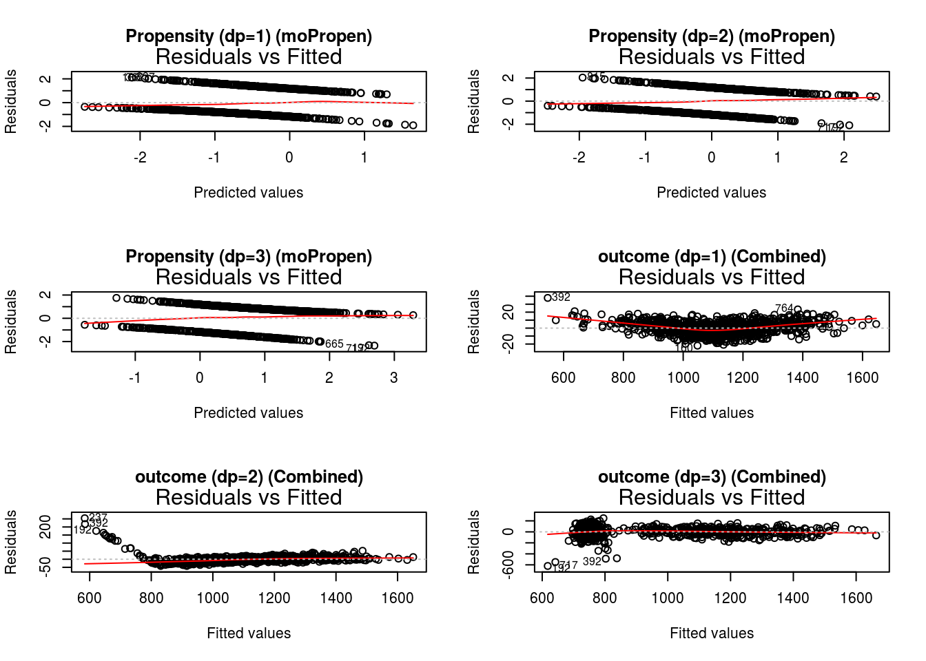
DynTxRegime::plot(x = result, suppress = TRUE, which = 1)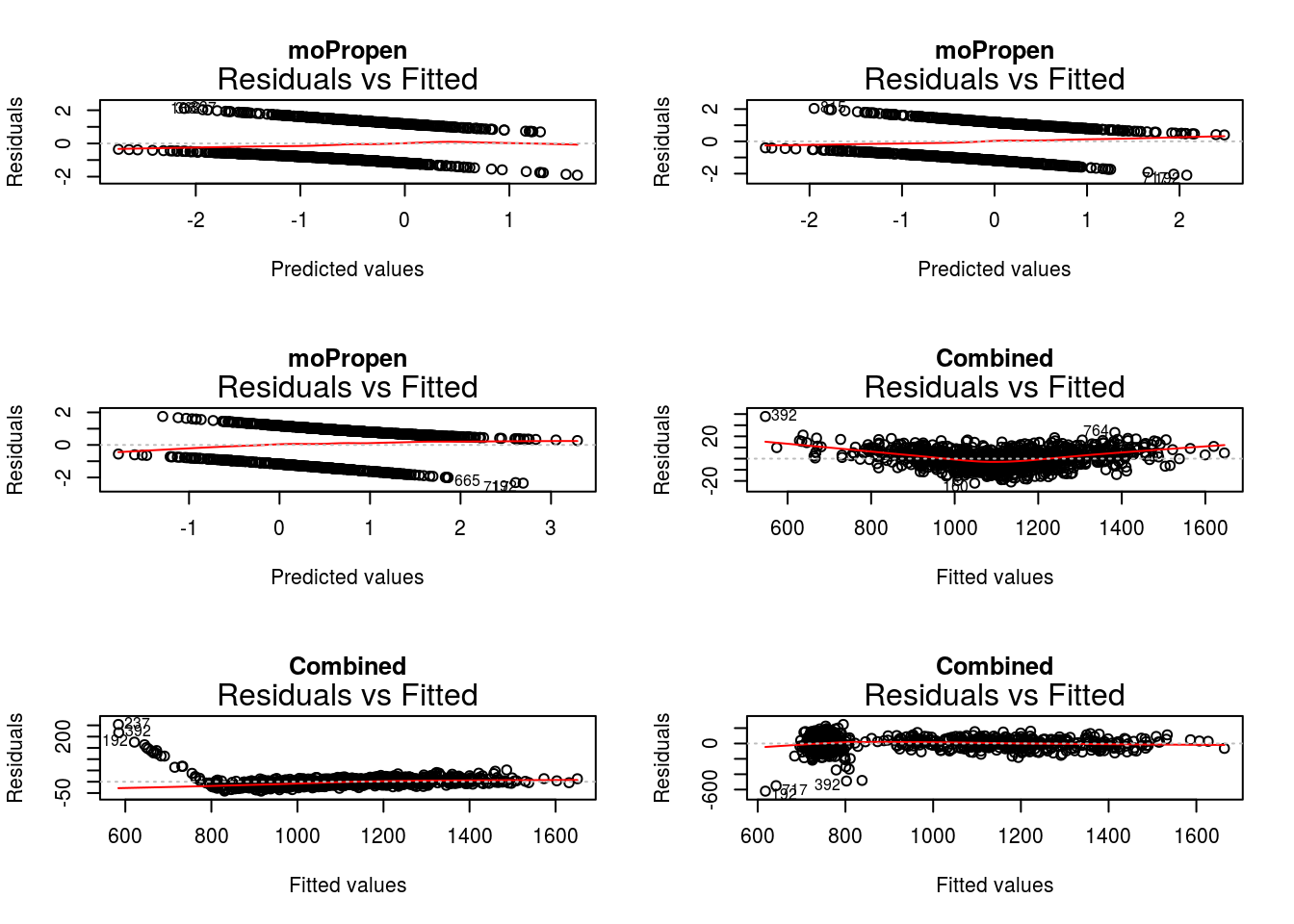
If there are additional diagnostic tools defined for a regression method used in the analysis but not implemented in DynTxRegime, the value object returned by the regression method can be extracted using function DynTxRegime::
fitObj <- DynTxRegime::fitObject(object = result)
fitObj$propensity
$propensity$`dp=1`
Call: glm(formula = YinternalY ~ CD4_0, family = "binomial", data = data)
Coefficients:
(Intercept) CD4_0
2.385956 -0.006661
Degrees of Freedom: 999 Total (i.e. Null); 998 Residual
Null Deviance: 1316
Residual Deviance: 1227 AIC: 1231
$propensity$`dp=2`
Call: glm(formula = YinternalY ~ CD4_6, family = "binomial", data = data)
Coefficients:
(Intercept) CD4_6
3.34284 -0.00609
Degrees of Freedom: 999 Total (i.e. Null); 998 Residual
Null Deviance: 1386
Residual Deviance: 1266 AIC: 1270
$propensity$`dp=3`
Call: glm(formula = YinternalY ~ CD4_12, family = "binomial", data = data)
Coefficients:
(Intercept) CD4_12
3.957186 -0.007436
Degrees of Freedom: 999 Total (i.e. Null); 998 Residual
Null Deviance: 1310
Residual Deviance: 1202 AIC: 1206
$outcome
$outcome$`dp=1`
$outcome$`dp=1`$Combined
Call:
lm(formula = YinternalY ~ CD4_0 + A1 + CD4_0:A1, data = data)
Coefficients:
(Intercept) CD4_0 A1 CD4_0:A1
362.86555 1.66681 17.00234 -0.04066
$outcome$`dp=2`
$outcome$`dp=2`$Combined
Call:
lm(formula = YinternalY ~ CD4_0 + CD4_6 + A2 + CD4_6:A2, data = data)
Coefficients:
(Intercept) CD4_0 CD4_6 A2 CD4_6:A2
337.5934 0.6360 0.8619 59.9512 -0.1110
$outcome$`dp=3`
$outcome$`dp=3`$Combined
Call:
lm(formula = YinternalY ~ CD4_0 + CD4_6 + CD4_12 + A3 + CD4_12:A3,
data = data)
Coefficients:
(Intercept) CD4_0 CD4_6 CD4_12 A3 CD4_12:A3
325.7049 0.6332 -0.0457 1.1595 507.3799 -1.9294 As for DynTxRegime::
is(object = fitObj$propensity$'dp=1')[1] "glm" "lm" "oldClass"As such, these objects can be passed to any tool defined for these classes. For example, the methods available for the object returned by the propensity regression are
utils::methods(class = is(object = fitObj$propensity$'dp=1')[1L]) [1] add1 anova coerce confint cooks.distance deviance drop1 effects extractAIC family formula
[12] influence initialize logLik model.frame nobs predict print residuals rstandard rstudent show
[23] slotsFromS3 summary vcov weights
see '?methods' for accessing help and source codeSo, to plot the residuals
graphics::plot(x = residuals(object = fitObj$propensity$'dp=1'))
Or, to retrieve the variance-covariance matrix of the parameters
stats::vcov(object = fitObj$propensity$'dp=1') (Intercept) CD4_0
(Intercept) 0.112867870 -2.49976e-04
CD4_0 -0.000249976 5.77706e-07The methods DynTxRegime::
DynTxRegime::propen(object = result)$`dp=1`
Call: glm(formula = YinternalY ~ CD4_0, family = "binomial", data = data)
Coefficients:
(Intercept) CD4_0
2.385956 -0.006661
Degrees of Freedom: 999 Total (i.e. Null); 998 Residual
Null Deviance: 1316
Residual Deviance: 1227 AIC: 1231
$`dp=2`
Call: glm(formula = YinternalY ~ CD4_6, family = "binomial", data = data)
Coefficients:
(Intercept) CD4_6
3.34284 -0.00609
Degrees of Freedom: 999 Total (i.e. Null); 998 Residual
Null Deviance: 1386
Residual Deviance: 1266 AIC: 1270
$`dp=3`
Call: glm(formula = YinternalY ~ CD4_12, family = "binomial", data = data)
Coefficients:
(Intercept) CD4_12
3.957186 -0.007436
Degrees of Freedom: 999 Total (i.e. Null); 998 Residual
Null Deviance: 1310
Residual Deviance: 1202 AIC: 1206DynTxRegime::genetic(object = result)$value
[1] 1169.871
$par
[1] 163.4563 175.6241 200.5718
$gradients
[1] NA NA NA
$generations
[1] 14
$peakgeneration
[1] 3
$popsize
[1] 1000
$operators
[1] 122 125 125 125 125 126 125 126 0Once satisfied that the postulated model is suitable, the estimated optimal treatment regime, the recommended treatments, and the estimated value for the dataset used for the analysis can be retrieved.
The estimated optimal treatment regime is retrieved using function DynTxRegime::
DynTxRegime::regimeCoef(object = result)$`dp=1`
eta1
163.4563
$`dp=2`
eta2
175.6241
$`dp=3`
eta3
200.5718 Function DynTxRegime::
DynTxRegime::optTx(x = result)$`dp=1`
$`dp=1`$optimalTx
[1] 0 0 0 0 0 0 0 0 0 0 0 0 0 0 0 0 0 0 0 0 0 0 0 0 0 0 0 0 0 0 0 0 0 0 0 0 0 0 0 0 0 0 0 0 0 0 0 0 0 0 0 0 0 0 0 0 0 0 0 0 0 0 0 0 0 0 0 0 0 0 0 0 0 0 0 0 0 0 0 0 0 0 0 0 0 0
[87] 0 0 0 0 0 0 0 0 0 0 0 0 0 0 0 0 0 0 0 0 0 0 0 0 0 0 0 0 0 0 0 0 0 0 0 0 0 0 0 0 0 0 0 0 0 0 0 0 0 0 0 0 0 0 0 0 0 0 0 0 0 0 0 0 0 0 0 0 0 0 0 0 0 0 0 0 0 0 0 0 0 0 0 0 0 0
[173] 0 0 0 0 0 0 0 0 0 0 0 0 0 0 0 0 0 0 0 0 0 0 0 0 0 0 0 0 0 0 0 0 0 0 0 0 0 0 0 0 0 0 0 0 0 0 0 0 0 0 0 0 0 0 0 0 0 0 0 0 0 0 0 0 1 0 0 0 0 0 0 0 0 0 0 0 0 0 0 0 0 0 0 0 0 0
[259] 0 0 0 0 0 0 0 0 0 0 0 0 0 0 0 0 0 0 0 0 0 0 0 0 0 0 0 0 0 0 0 0 0 0 0 0 0 0 0 0 0 0 0 0 0 0 0 0 0 0 0 0 0 0 0 0 0 0 0 0 0 0 0 0 0 0 0 0 0 0 0 0 0 0 0 0 0 0 0 0 0 0 0 0 0 0
[345] 0 0 0 0 0 0 0 0 0 0 0 0 0 0 0 0 0 0 0 0 0 0 0 0 0 0 0 0 0 0 0 0 0 0 0 0 0 0 0 0 0 0 0 0 0 0 0 1 0 0 0 0 0 0 0 0 0 0 0 0 0 0 0 0 0 0 0 0 0 0 0 0 0 0 0 0 0 0 0 0 0 0 0 0 0 0
[431] 0 0 0 0 0 0 0 0 0 0 0 0 0 0 0 0 0 0 0 0 0 0 0 0 0 0 0 0 0 0 0 0 0 0 0 0 0 0 0 0 0 0 0 0 0 0 0 0 0 0 0 0 0 0 0 0 0 0 0 0 0 0 0 0 0 0 0 0 0 0 0 0 0 0 0 0 0 0 0 0 0 0 0 0 0 0
[517] 0 0 0 0 0 0 0 0 0 0 0 0 0 0 0 0 0 0 0 0 0 0 0 0 0 0 0 0 0 0 0 0 0 0 0 0 0 0 0 0 0 0 0 0 0 0 0 0 0 0 0 0 0 0 0 0 0 0 0 0 0 0 0 0 0 0 0 0 0 0 0 0 0 0 0 0 0 0 0 0 0 0 0 0 0 0
[603] 0 0 0 0 0 0 0 0 0 0 0 0 0 0 0 0 0 0 0 0 0 0 0 0 0 0 0 0 0 0 0 0 0 0 0 0 0 0 0 0 0 0 0 0 0 0 0 0 0 0 0 0 0 0 0 0 0 0 0 0 0 0 0 0 0 0 0 0 0 0 0 0 0 0 0 0 0 0 0 0 0 0 0 0 0 0
[689] 0 0 0 0 0 0 0 0 0 0 0 0 0 0 0 0 0 0 0 0 0 0 0 0 0 0 0 0 0 0 0 0 0 0 0 0 0 0 0 0 0 0 0 0 0 0 0 0 0 0 0 0 0 0 0 0 0 0 0 0 0 0 0 0 0 0 0 0 0 0 0 0 0 0 0 0 0 0 0 0 0 0 0 0 0 0
[775] 0 0 0 0 0 0 0 0 0 0 0 0 0 1 0 0 0 0 0 0 0 0 0 0 0 0 0 0 0 0 0 0 0 0 0 0 0 0 0 0 0 0 0 0 0 0 0 0 0 0 0 0 0 0 0 0 0 0 0 0 0 0 0 0 0 0 0 0 0 0 0 0 0 0 0 0 0 0 0 0 0 0 0 0 0 0
[861] 0 0 0 0 0 0 0 0 0 0 0 0 0 0 0 0 0 0 0 0 0 0 0 0 0 0 0 0 0 0 0 0 0 0 0 0 0 0 0 0 1 0 0 0 0 0 0 0 0 0 0 0 0 0 0 0 0 0 0 0 0 0 0 0 0 0 0 0 0 0 0 0 0 0 0 0 0 0 0 0 0 0 0 0 0 0
[947] 0 0 0 0 0 0 0 0 0 0 0 0 0 0 0 0 0 0 0 0 0 0 0 0 0 0 0 0 0 0 0 0 0 0 0 0 0 0 0 0 0 0 0 0 0 0 0 0 0 0 0 0 0 0
$`dp=1`$decisionFunc
[1] NA
$`dp=2`
$`dp=2`$optimalTx
[1] 0 0 0 0 0 0 0 0 0 0 0 0 0 0 0 0 0 0 0 0 0 0 0 0 0 0 0 0 0 0 0 0 0 0 0 0 0 0 0 0 0 0 0 0 0 0 0 0 0 0 0 0 0 0 0 0 0 0 0 0 0 0 0 0 0 0 0 0 0 0 0 0 0 0 0 0 0 0 0 0 0 0 0 0 0 0
[87] 0 0 0 0 0 0 0 0 0 0 0 0 0 0 0 0 0 0 0 0 0 0 0 0 0 0 0 0 0 0 0 0 0 0 0 0 0 0 0 0 0 0 0 0 0 0 0 0 0 0 0 0 0 0 0 0 0 0 0 0 0 0 0 0 0 0 0 0 0 0 0 0 0 0 0 0 0 0 0 0 0 0 0 0 0 0
[173] 0 0 0 0 0 0 0 0 0 0 0 0 0 0 0 0 0 0 0 0 0 0 0 0 0 0 0 0 0 0 0 0 0 0 0 0 0 0 0 0 0 0 0 0 0 0 0 0 0 0 0 0 0 0 0 0 0 0 0 0 0 0 0 0 1 0 0 0 0 0 0 0 0 0 0 0 0 0 0 0 0 0 0 0 0 0
[259] 0 0 0 0 0 0 0 0 0 0 0 0 0 0 0 0 0 0 0 0 0 0 0 0 0 0 0 0 0 0 0 0 0 0 0 0 0 0 0 0 0 0 0 0 0 0 0 0 0 0 0 0 0 0 0 0 0 0 0 0 0 0 0 0 0 0 0 0 0 0 0 0 0 0 0 0 0 0 0 0 0 0 0 0 0 0
[345] 0 0 0 0 0 0 0 0 0 0 0 0 0 0 0 0 0 0 0 0 0 0 0 0 0 0 0 0 0 0 0 0 0 0 0 0 0 0 0 0 0 0 0 0 0 0 0 1 0 0 0 0 0 0 0 0 0 0 0 0 0 0 0 0 0 0 0 0 0 0 0 0 0 0 0 0 0 0 0 0 0 0 0 0 0 0
[431] 0 0 0 0 0 0 0 0 0 0 0 0 0 0 0 0 0 0 0 0 0 0 0 0 0 0 0 0 0 0 0 0 0 0 0 0 0 0 0 0 0 0 0 0 0 0 0 0 0 0 0 0 0 0 0 0 0 0 0 0 0 0 0 0 0 0 0 0 0 0 0 0 0 0 0 0 0 0 0 0 0 0 0 0 0 0
[517] 0 0 0 0 0 0 0 0 0 0 0 0 0 0 0 0 0 0 0 0 0 0 0 0 0 0 0 0 0 0 0 0 0 0 0 0 0 0 0 0 0 0 0 0 0 0 0 0 0 0 0 0 0 0 0 0 0 0 0 0 0 0 0 0 0 0 0 0 0 0 0 0 0 0 0 0 0 0 0 0 0 0 0 0 0 0
[603] 0 0 0 0 0 0 0 0 0 0 0 0 0 0 0 0 0 0 0 0 0 0 0 0 0 0 0 0 0 0 0 0 0 0 0 0 0 0 0 0 0 0 0 0 0 0 0 0 0 0 0 0 0 0 0 0 0 0 0 0 0 0 0 0 0 0 0 0 0 0 0 0 0 0 0 0 0 0 0 0 0 0 0 0 0 0
[689] 0 0 0 0 0 0 0 0 0 0 0 0 0 0 0 0 0 0 0 0 0 0 0 0 0 0 0 0 0 0 0 0 0 0 0 0 0 0 0 0 0 0 0 0 0 0 0 0 0 0 0 0 0 0 0 0 0 0 0 0 0 0 0 0 0 0 0 0 0 0 0 0 0 0 0 0 0 0 0 0 0 0 0 0 0 0
[775] 0 0 0 0 0 0 0 0 0 0 0 0 0 1 0 0 0 0 0 0 0 0 0 0 0 0 0 0 0 0 0 0 0 0 0 0 0 0 0 0 0 0 0 0 0 0 0 0 0 0 0 0 0 0 0 0 0 0 0 0 0 0 0 0 0 0 0 0 0 0 0 0 0 0 0 0 0 0 0 0 0 0 0 0 0 0
[861] 0 0 0 0 0 0 0 0 0 0 0 0 0 0 0 0 0 0 0 0 0 0 0 0 0 0 0 0 0 0 0 0 0 0 0 0 0 0 0 0 1 0 0 0 0 0 0 0 0 0 0 0 0 0 0 0 0 0 0 0 0 0 0 0 0 0 0 0 0 0 0 0 0 0 0 0 0 0 0 0 0 0 0 0 0 0
[947] 0 0 0 0 0 0 0 0 0 0 0 0 0 0 0 0 0 0 0 0 0 0 0 0 0 0 0 0 0 0 0 0 0 0 0 0 0 0 0 0 0 0 0 0 0 0 0 0 0 0 0 0 0 0
$`dp=2`$decisionFunc
[1] NA
$`dp=3`
$`dp=3`$optimalTx
[1] 0 0 0 0 0 0 0 0 0 0 0 0 0 0 0 0 0 0 0 0 0 0 0 0 0 0 0 0 0 0 0 0 0 0 0 0 0 0 0 0 0 0 0 0 0 0 0 0 0 0 0 0 0 0 0 0 0 0 0 0 0 0 0 0 0 0 0 0 0 0 0 0 0 0 0 0 0 0 0 0 0 0 0 0 0 0
[87] 0 0 0 0 0 0 0 0 0 0 0 0 0 0 0 0 0 0 0 0 0 0 0 0 0 0 0 0 0 0 0 0 0 0 0 0 0 0 0 0 0 0 0 0 0 0 0 0 0 0 0 0 0 0 0 0 0 0 0 0 0 0 0 0 0 0 0 0 0 0 0 0 0 0 0 0 0 0 0 0 0 0 0 0 0 0
[173] 0 0 0 0 0 0 0 0 1 0 0 0 0 0 0 0 0 0 0 1 0 0 0 0 0 0 0 0 0 0 0 0 0 0 0 0 0 0 0 0 0 0 0 0 0 0 0 0 0 0 0 0 0 0 0 0 0 0 0 0 0 0 0 0 1 0 0 0 0 0 0 0 0 0 0 0 0 0 0 0 0 0 0 0 0 0
[259] 0 0 0 0 0 0 0 0 0 0 0 0 0 0 0 0 0 0 0 0 0 0 0 0 0 0 0 0 0 0 0 0 0 0 0 0 0 0 0 0 0 0 0 0 0 0 0 0 0 0 0 0 0 0 0 0 0 0 0 0 0 0 0 0 0 0 0 0 0 0 0 0 0 0 0 0 0 0 0 0 0 0 0 0 0 0
[345] 0 0 0 0 0 0 0 0 0 0 0 0 0 0 0 0 0 0 0 0 0 0 0 0 0 0 0 0 0 0 0 0 0 0 0 0 0 1 0 0 0 0 0 0 0 0 0 1 0 0 0 0 0 0 0 0 0 0 0 0 0 0 0 0 0 0 0 0 0 0 0 0 0 0 0 0 0 0 0 0 0 0 0 0 0 0
[431] 0 0 0 0 0 0 0 0 0 0 0 0 0 0 0 0 0 0 0 0 0 0 0 0 0 0 0 0 0 0 0 0 0 0 0 0 0 0 0 0 0 0 0 0 0 0 0 0 0 0 0 0 0 0 0 0 1 0 0 0 0 0 0 0 0 0 0 0 0 0 0 0 0 0 0 0 0 0 0 0 0 0 0 0 0 0
[517] 1 0 0 0 0 0 0 0 0 0 0 0 0 0 0 0 0 0 0 0 0 0 0 0 0 0 0 0 0 0 0 0 0 0 0 0 0 0 0 0 0 1 0 0 0 0 0 0 0 0 0 0 0 0 0 0 0 0 0 0 0 0 0 0 0 0 0 0 0 0 0 0 0 0 0 0 0 0 0 0 0 0 0 0 0 0
[603] 0 0 0 0 0 0 0 0 0 0 0 0 0 0 0 0 0 0 0 0 0 0 0 0 0 0 0 0 0 0 0 0 0 0 0 0 0 0 0 0 0 0 0 0 0 0 0 0 0 0 0 0 0 0 0 0 0 0 0 0 0 0 0 0 0 0 0 0 0 0 0 0 0 0 0 0 0 0 0 0 0 0 0 0 0 0
[689] 0 0 0 0 0 0 0 0 0 0 0 0 0 0 0 0 0 0 0 0 0 0 0 0 0 0 0 0 1 0 0 0 0 0 0 0 0 0 0 0 0 0 0 0 0 0 0 0 0 0 0 0 0 0 0 0 0 0 0 0 0 0 0 0 0 0 0 0 0 0 0 0 0 0 0 0 0 0 0 0 0 0 0 0 0 0
[775] 0 0 0 0 0 0 0 0 0 0 0 0 0 1 0 0 0 0 0 0 0 0 0 0 0 0 0 0 0 0 0 0 0 0 0 0 0 0 0 0 0 0 0 0 0 0 0 0 0 0 0 0 0 0 0 0 0 0 0 0 0 0 0 0 0 0 0 0 0 0 0 0 0 0 0 0 0 0 0 0 0 0 0 0 0 0
[861] 0 0 0 0 0 0 0 0 0 0 0 0 0 0 0 0 0 0 0 0 0 0 0 0 0 0 0 0 0 0 0 0 0 0 0 0 0 0 0 0 1 0 0 0 0 0 0 0 0 0 0 0 0 0 0 0 0 0 0 0 0 0 0 0 0 0 0 0 0 0 0 0 0 0 0 0 0 0 0 0 0 0 0 0 0 0
[947] 0 0 1 0 0 0 0 0 0 0 0 0 0 0 0 0 0 0 0 0 1 0 0 0 0 0 0 0 0 0 0 0 0 0 0 0 0 0 0 0 0 0 0 0 0 0 0 0 0 0 0 0 0 0
$`dp=3`$decisionFunc
[1] NAThe object returned is a list of lists. The outermost list indicates the decision point to which the results pertain. The inner list contains element $optimalTx, which corresponds to the \(\widehat{d}^{opt}_{\eta}(H_{1i}; \widehat{\eta}_{1})\), and element $decisionFunc, which is not defined in this context and thus is NA; it is included for continuity across methods.
Function DynTxRegime::
DynTxRegime::estimator(x = result)[1] 1169.871
Function DynTxRegime::
The first new patient has the following baseline covariates
print(x = patient1) CD4_0
1 457The recommended treatment based on the previous first stage analysis is obtained by providing the object returned by optimalSeq() as well as a ‘data.frame’ object that contains the baseline covariates of the new patient.
DynTxRegime::optTx(x = result, newdata = patient1, dp = 1L)$optimalTx
[1] 0
$decisionFunc
[1] NATreatment A1= 0 is recommended.
Assume that patient1 receives the recommended first stage treatment, and \(x_{2}\) is measured six months after treatment. The available history is now
print(x = patient1) CD4_0 A1 CD4_6
1 457 0 576.9The recommended treatment based on the previous second stage analysis is obtained by providing the object returned by optimalSeq() as well as a ‘data.frame’ object that contains the available covariates and treatment history of the new patient.
DynTxRegime::optTx(x = result, newdata = patient1, dp = 2L)$optimalTx
[1] 0
$decisionFunc
[1] NATreatment A2= 0 is recommended.
Again, patient1 receives the recommended treatment, and \(x_{3}\) is measured six months after treatment. The available history is now
print(x = patient1) CD4_0 A1 CD4_6 A2 CD4_12
1 457 0 576.9 0 460.6Finally recommended treatment based on the previous third stage analysis is obtained by providing the object returned by optimalSeq() as well as a ‘data.frame’ object that contains the available covariates and treatment history of the new patient.
DynTxRegime::optTx(x = result, newdata = patient1, dp = 3L)$optimalTx
[1] 0
$decisionFunc
[1] NATreatment A3= 0 is recommended.
Note that though the estimated optimal treatment regime was obtained starting at stage K and ending at stage 1, predicted optimal treatment regimes for new patients clearly must be obtained starting at the first stage. Predictions for subsequent stages cannot be obtained until the mid-stage covariate information becomes available.
Classification Estimator
The multiple decision point classification algorithm can be viewed as the application of the classification method of a single decision optimal regime discussed previously in Chapter 4 within the framework of the backward iterative algorithm.
Let
\[ \begin{align} \widehat{\mathcal{V}}_{AIPW}^{(K)}(d_{\eta,K}) &= n^{-1} \sum_{i=1}^{n}~\left[ \mathcal{G}_{AIPW,Ki}(1;\widehat{\gamma}_{K}, \widehat{\beta}_{K}) \text{I}\{d_{\eta,K}(H_{Ki}) = 1\} + \mathcal{G}_{AIPW,Ki}(0;\widehat{\gamma}_{K}, \widehat{\beta}_{K}) \text{I}\{d_{\eta,K}(H_{Ki}) = 0\}\right], \end{align} \] where \[ \begin{align} \mathcal{G}_{AIPW,Ki}(a_{K};\widehat{\gamma}_{K}, \widehat{\beta}_{K}) =& \frac{ \text{I} \{ A_{Ki} = a_{K}\} Y_{i} }{\omega_{K}(H_{Ki}, A_{Ki};\widehat{\gamma}_{K}) } - \left[ \frac{ \text{I}\{ A_{Ki} = a_{K}\} - \omega_{K}(H_{Ki}, A_{Ki}; \widehat{\gamma}_{K})} { \omega_{K}(H_{Ki}, A_{Ki}; \widehat{\gamma}_{K}) } \right] Q_{K}^{{d_{\eta}}}(H_{Ki},a_{K}; \widehat{\beta}_K); \end{align} \] \(Q_{K}^{d_{\eta}}(h_{K},a_{K};\beta_{K})\) is a model for \(E(Y|H_{K} = h_{K}, A_{K} = a_{K})\); \(\omega_{k}(h_{k}, a_{k}; \widehat{\gamma}_{k})\) is a model for
\[ \omega_{k}(h_{k},a_{k}) = \sum_{l = 1}^{l_{k}} \text{I}\{s_{k}(h_{k}) = l\}~\omega_{k,l}(h_{k},a_{k}) \quad k = 1, \dots, K; \] \(\omega_{k,l}(h_{k},a_{k}) = P(A_{k} = a_{k}|H_{k} = h_{k})\); and \(\widehat{\beta}_{k}\) and \(\widehat{\gamma}_{k}\) are suitable estimators for \(\beta_{k}\) and \(\gamma_{k}\), respectively.
This value estimator has the form of an augmented inverse probability weighted estimator for a single decision problem, with Decision \(K\) and \(d_{\eta,K}\) playing the roles of the single decision point and the corresponding single decision rule, respectively. All other covariates and previous treatments received are considered to be `baseline’ covariates.
The first step of the backward algorithm is to maximize \(\widehat{\mathcal{V}}^{(K)}_{AIPW}(d_{\eta,K})\) in \(\eta_{K}\) to obtain \(\widehat{\eta}^{opt}_{K,B,AIPW}\) and thus to estimate \(d^{opt}_{\eta,K,B}(h_{K}) = d_{K}(h_{K};\widehat{\eta}^{opt}_{K,B,AIPW})\).
The maximization step is likened to a weighted classification problem in a manner similar to that used for the single decision probelm. Specifically, the classification estimator is obtained by minimizing in \(\eta_K\)
\[ \begin{align} n^{-1} \sum_{i=1}^{n} \left| \widehat{C}_{Ki} \right|~ \text{I}\left\{ \text{I}(\widehat{C}_{Ki} \geq 0 ) \neq d_{K}(H_{Ki}; \eta_{K})\right\}, \end{align} \]
where \(\widehat{C}_{Ki}\) is defined as
\[ \widehat{C}_{Ki} = \mathcal{G}_{AIPW,Ki}(1;\widehat{\gamma}_{K}, \widehat{\beta}_{K}) - \mathcal{G}_{AIPW,Ki}(0;\widehat{\gamma}_{K}, \widehat{\beta}_{K}). \]
Comparison of the expression to be minimized to the standard weighted classification error of the generic classification problem shows that \(\left| \widehat{C}_{Ki}\right|\) can be identified as the “weight”, \(\text{I}\{ \widehat{C}_{Ki} \geq 0\}\) as the “label,” and \(d_{K}(H_{Ki}; \eta_{K})\) as the “classifier.” There are many well-established methods to solve this minimization problem and obtain \(\widehat{\eta}^{opt}_{K,B,AIPW}\).
For notational convenience here, we define pseudo outcomes \[
\begin{align}
\widetilde{V}^{d_{\eta}}_{Ki} &=
\mathcal{G}_{AIPW,Ki}(1;\widehat{\gamma}_{K}, \widehat{\beta}_{K}) \text{I}\{\widehat{d}_{\eta,K,B}^{opt}(H_{Ki}) = 1\} + \mathcal{G}_{AIPW,Ki}(0;\widehat{\gamma}_{K}, \widehat{\beta}_{K}) \text{I}\{\widehat{d}_{\eta,K,B}^{opt}(H_{Ki}) = 0\} \end{align}
\]
and for Decision K-1 maximize in \(\eta_{K-1}\)
\[ \begin{align} \widehat{\mathcal{V}}_{AIPW}^{(K-1)}(d_{\eta,K-1},d_{\eta,K}) &= n^{-1} \sum_{i=1}^{n}~\left[ \mathcal{G}_{AIPW,K-1,i}(1;\widehat{\gamma}_{K-1}, \widehat{\beta}_{K-1}) \text{I}\{d_{\eta,K-1}(H_{K-1,i}) = 1\} \right.\\ & \left. + \mathcal{G}_{AIPW,K-1,i}(0;\widehat{\gamma}_{K-1}, \widehat{\beta}_{K-1}) \text{I}\{d_{\eta,K-1}(H_{K-1,i}) = 0\}\right], \end{align} \] where for \(k = K-1, \dots, 1\)
\[ \begin{align} \mathcal{G}_{AIPW,ki}(a_{k};\widehat{\gamma}_{k}, \widehat{\beta}_{k}) =& n^{-1} \sum_{i=1}^{n}~~ \frac{ \text{I} \{ A_{ki} = a_{k}\} {V}^{d_{\eta}}_{k+1,i}} {\omega_{k}(H_{ki}, A_{ki};\widehat{\gamma}_{k}) } - \left[ \frac{ \text{I}\{ A_{ki} = a_{k}\} - \omega_{k}(H_{ki}, A_{ki}; \widehat{\gamma}_{k})} { \omega_{k}(H_{ki}, A_{ki}; \widehat{\gamma}_{k}) } \right] Q_{k}^{{d_{\eta}}}\{H_{ki},a_{k}; \widehat{\beta}_k\}. \end{align} \]
As for Decision \(K\), this maximization can be likened to a weighted classification problem, and the classification estimator is obtained by minimizing in \(\eta_{K-1}\)
\[ \begin{align} n^{-1} \sum_{i=1}^{n} \left| \widehat{C}_{K-1,i} \right|~ \text{I}\left\{ \text{I}(\widehat{C}_{K-1,i} \geq 0 ) \neq d_{K-1}(H_{K-1,i}; \eta_{K-1})\right\}, \end{align} \]
where \(\widehat{C}_{ki}, k=, K-1, \dots, 1\) is defined as
\[ \widehat{C}_{ki} = \mathcal{G}_{AIPW,ki}(1;\widehat{\gamma}_{k}, \widehat{\beta}_{k}) - \mathcal{G}_{AIPW,ki}(0;\widehat{\gamma}_{k}, \widehat{\beta}_{k}). \]
The procedure of maximizing \(\widehat{\mathcal{V}}_{AIPW}^{(k)}(d_{\eta,k})\) to obtain \(\widehat{\eta}_{k,B,AIPW}\) and thus \(\widehat{d}^{opt}_{\eta,k,B}(h_{k})\) is continued for \(k = K-2, \dots, 1\).
The IPW estimator is the special case of specifying \(Q_{k}(h_{k},a_{k}) \equiv 0, k = 1, \dots, K\).
A general implementation of the classification estimator is provided in
The function call for DynTxRegime::
utils::str(object = DynTxRegime::optimalClass)function (..., moPropen, moMain, moCont, moClass, data, response, txName, iter = 0L, fSet = NULL, verbose = TRUE) We briefly describe the input arguments for DynTxRegime::
| Input Argument | Description |
|---|---|
| \(\dots\) | Ignored; included only to require named inputs. |
| moPropen | A “modelObj” object or a list of “modelObj” objects. The modeling object(s) for the \(k^{th}\) propensity regression step. |
| moMain | A “modelObj” object or a list of “modelObj” objects. The modeling object(s) for the \(\nu_{k}(h_{k}; \phi_{k})\) component of \(Q_{k}(h_{k},a_{k};\beta_{k})\). |
| moCont | A “modelObj” object or a list of “modelObj” objects. The modeling object(s) for the \(\text{C}_{k}(h_{k}; \psi_{k})\) component of \(Q_{k}(h_{k},a_{k};\beta_{k})\). |
| moClass | A “modelObj” object. The modeling object(s) for the \(k^{th}\) classification regression step. |
| data | A “data.frame” object. The covariate history and the treatments received. |
| response | For Decision K analysis, a “numeric” vector. The outcome of interest, where larger values are better. For analysis of Decision k, k = 1, …, K-1, an “OptimalClass” object. The value object returned by |
| txName | A “character” object. The column header of data corresponding to the \(k^{th}\) stage treatment variable. |
| iter | An “integer” object. The maximum number of iterations for iterative algorithm. |
| fSet | A “function”. A user defined function specifying treatment or model subset structure of Decision \(k\). |
| verbose | A “logical” object. If TRUE progress information is printed to screen. |
Methods implemented in DynTxRegime break the Q-function model into two components: a main effects component and a contrasts component. For example, for binary treatments, \(Q_{k}(h_{k}, a_{k}; \beta_{k})\) can be written as
\[ Q_{k}(h_{k}, a_{k}; \beta_{k})= \nu_{k}(h_{k}; \phi_{k}) + a_{k} \text{C}_{k}(h_{k}; \psi_{k}), \text{for} ~ k = 1, \dots, K \]
where \(\beta_{k} = (\phi^{\intercal}_{k}, \psi^{\intercal}_{k})^{\intercal}\). Here, \(\nu_{k}(h_{k}; \phi_{k})\) comprises the terms of the model that are independent of treatment (so called “main effects” or “common effects”), and \(\text{C}_{k}(h_{k}; \psi_{k})\) comprises the terms of the model that interact with treatment (so called “contrasts”). Input arguments moMain and moCont specify \(\nu_{k}(h_{k}; \phi_{k})\) and \(\text{C}_{k}(h_{k}; \psi_{k})\), respectively.
In the examples provided in this chapter, the two components of each \(Q_{k}(h_{k}, a_{k}; \beta_{k})\) are both linear models, the parameters of which are estimated using stats::
Input fSet is a user-defined function specifying the feasible sets. The only requirements for this input are:
- The formal input argument(s) of the function must be either data or the individual covariates required for identifying subset membership.
- The function must return a list containing two elements $subsets and $txOpts.
Element $subsets of the returned list is itself a list; each element of the list contains a nickname and the treatment options for a single feasible set.
Element $txOpts of the returned list is a character vector providing the nickname of the feasible set to which each individual is assigned. - There are no requirements for the function name or the structure of the function contents.
See the Analysis tab for explicit examples.
The value object returned by DynTxRegime::
| Slot Name | Description |
|---|---|
| @step | An integer indicating the step of the backward iterative algorithm. |
| @analysis@classif | The classification results. |
| @analysis@outcome | The outcome regression analysis if AIPW value estimator; NA if IPW. |
| @analysis@propen | The propensity score regression analysis. |
| @analysis@call | The unevaluated function call. |
| @analysis@optimal | The estimated value and optimal treatment for the training data. |
There are several methods available for objects of this class that assist with model diagnostics, the exploration of training set results, and the estimation of optimal treatments for future patients. We explore some of these methods in the Methods section.
Both the simple and augmented inverse probability weighted value estimators can be used for DynTxRegime::
The backward iterative algorithm begins with the analysis of Decision \(K\). In our current example, \(K=3\).
Input moPropen is a modeling object or a list of modeling objects specifying the \(l\) subset model(s) for \(\omega_{3}(h_{3},a_{3})\). In this example, \(l=2\). However, individuals that previously received treatment 1 (i.e., those for whom \(s_{3}(h_{3}) = 1\)) remain on treatment 1 with probability 1.0, and a model is not posited or fitted for this subset. Thus only one modeling object is needed. We posit the following model for individuals in feasible set \(s_{3}(h_{3}) = 2\)
\[ \text{logit}\left\{\omega_{3,2}(h_{3},1;\gamma_{3})\right\} = \gamma_{30} + \gamma_{31}~\text{CD4_12}, \]
where \(\text{logit}(p) = \text{log} \{p/(1-p)\}\). The modeling object for this model is
p3 <- modelObj::buildModelObj(model = ~ CD4_12,
solver.method = 'glm',
solver.args = list(family='binomial'),
predict.method = 'predict.glm',
predict.args = list(type='response'))Inputs moMain and moCont are modeling objects specifying the model posited for \(Q_{3}(h_3, a_3) = E(Y|\overline{X} = \overline{x}, \overline{A} = \overline{a})\). We posit the following model
\[ Q_{3}(h_{3},a_{3};{\beta}_{3}) = {\beta}_{30} + {\beta}_{31} \text{CD4_0} + {\beta}_{32} \text{CD4_6} + {\beta}_{33} \text{CD4_12} + a_{3}~({\beta}_{34} + {\beta}_{35} \text{CD4_12}), \]
the modeling objects of which are specified as
q3Main <- modelObj::buildModelObj(model = ~ CD4_0 + CD4_6 + CD4_12,
solver.method = 'lm',
predict.method = 'predict.lm')q3Cont <- modelObj::buildModelObj(model = ~ CD4_12,
solver.method = 'lm',
predict.method = 'predict.lm')Note that the formula in the contrast component does not contain the treatment variable; it contains only the covariate(s) that interact with the treatment.
Both components of the outcome regression model are of the same class, and the models should be fit as a single combined object. Thus, the iterative algorithm is not required, and iter should keep its default value.
To see a brief synopsis of the model diagnostics for this model, see header \(Q_{k}(h_{k},a_{k};\beta_{k})\) in the sidebar menu.
Input moClass is a modeling object that specifies the restricted class of regimes and the
library(rpart)
moC3 <- modelObj::buildModelObj(model = ~ CD4_12,
solver.method = 'rpart',
predict.args = list(type='class'))Notice that we have modified the default prediction arguments, predict.args, to ensure that predictions are returned as the class to which the record is assigned. For this method, predictions for the classification step must be the class.
The “data.frame” containing all covariates and treatments received is data set dataMDPF, the third stage treatment is contained in column $A3 of dataMDPF, and the outcome of interest is contained in column $Y.
Because not all treatments are available to all patients, we must define fSet, a function that defines the feasible sets and matches individuals to the appropriate feasible set. Specifically, the feasible sets for Decision 3 are defined to be
\[ \Psi_{3}(h_{3}) = \left\{ \begin{array}{cl} \{1\} \subset \mathcal{A}_{3} & \text{if } A_{2} = 1~\{s_{3}(h_{3}) = 1\}\\ \{ 0,1\} \subset \mathcal{A}_{3}& \text{if } A_{2} = 0~\{s_{3}(h_{3}) = 2\}\\ \end{array} \right. . \]
That is, individuals that received treatment \(A_{2}=1\) remain on treatment 1. All others are assigned one of \(A_{3} = \{0,1\}\). An example of a user-defined function that defines the feasible sets for Decision 3 is
fSet3 <- function(data){
subsets <- list(list("s1",1L),
list("s2",c(0L,1L)))
txOpts <- rep(x = 's2', times = nrow(x = data))
txOpts[data$A2 == 1L] <- "s1"
return(list("subsets" = subsets, "txOpts" = txOpts))
}Note that this is not the only possible function specification; there are innumerable ways to specify this rule in R. The only requirements for this input are that the formal input argument of the function must be data and that the function must return a list containing $subsets and $txOpts, which contain a list describing the feasible sets and a vector specifying the feasible set to which each patient is associated.
The optimal treatment rule for Decision 3, \(d_{3}(h_{3};\widehat{\eta}^{opt}_{3,B,AIPW})\), is estimated as follows.
class3 <- DynTxRegime::optimalClass(moPropen = p3,
moMain = q3Main,
moCont = q3Cont,
moClass = moC3,
data = dataMDPF,
response = dataMDPF$Y,
txName = "A3",
fSet = fSet3,
verbose = TRUE)AIPW value estimatorFirst step of the Classification Algorithm.Classification Perspective.
Subsets of treatment identified as:
$s1
[1] 1
$s2
[1] 0 1
Number of patients in data for each subset:
s1 s2
486 514
Propensity for treatment regression.subset s1 excluded from propensity regression514 included in analysis
Regression analysis for moPropen:
Call: glm(formula = YinternalY ~ CD4_12, family = "binomial", data = data)
Coefficients:
(Intercept) CD4_12
0.929409 -0.003816
Degrees of Freedom: 513 Total (i.e. Null); 512 Residual
Null Deviance: 622.5
Residual Deviance: 609.1 AIC: 613.1
Subsets of treatment identified as:
$s1
[1] 1
$s2
[1] 0 1
Number of patients in data for each subset:
s1 s2
486 514
Outcome regression.NOTE: subset(s) s1 excluded from outcome regressionCombined outcome regression model: ~ CD4_0+CD4_6+CD4_12 + A3 + A3:(CD4_12) .
514 included in analysis
Regression analysis for Combined:
Call:
lm(formula = YinternalY ~ CD4_0 + CD4_6 + CD4_12 + A3 + CD4_12:A3,
data = data)
Coefficients:
(Intercept) CD4_0 CD4_6 CD4_12 A3 CD4_12:A3
317.3743 2.0326 0.1371 -0.4478 603.5614 -1.9814
Classification Analysis
514 included in analysis
Regression analysis for moClass:
n= 514
node), split, n, loss, yval, (yprob)
* denotes terminal node
1) root 514 0.026513730 0 (0.9992587582 0.0007412418)
2) CD4_12>=330.8326 490 0.003890586 0 (0.9998900779 0.0001099221) *
3) CD4_12< 330.8326 24 0.009605578 1 (0.9397205655 0.0602794345)
6) CD4_12>=303.7734 13 0.003430213 0 (0.9800321814 0.0199678186) *
7) CD4_12< 303.7734 11 0.005020235 1 (0.9056939321 0.0943060679) *
Recommended Treatments:
0 1
503 497
Estimated value: 953.2091 Above, we opted to set verbose to TRUE to highlight some of the information that should be verified by a user. Notice the following:
- The first lines of the verbose output indicates that the selected analysis is a step of the classification method.
Users should verify that this is the intended step. If it is not, verify input response. - The feasible sets are summarized including the number of individuals assigned to each set.
Users should verify that input fSet was properly interpreted by the software. - The information provided for \(\omega_{k,l}(h_{k},a_{k};\gamma_{k})\), \(Q(h_{k},a_{k};\eta_{k})\), and the classification regressions are not defined within DynTxRegime::
optimalClass() , but is specified by the statistical method selected to obtain parameter estimates.
Users should verify that the model was correctly interpreted by the software and that there are no warnings or messages reported by the regression method. - Notice that only a subset of the data was used in the regression analysis. This reflects that only those individuals for whom more than one treatment option was available were included in the regression, i.e., only those for whom \(s_{3}(h_{3}) = 2\).
- Finally, a tabled summary of the recommended treatments and the estimated value for the training data are shown.
Recall that this estimated value is not the estimated value of the full optimal regime, but is the mean of the pseudo-outcomes \(\tilde{V}_{3}\).
The first step of the post-analysis should always be model diagnostics. DynTxRegime comes with several tools to assist in this task. However, we have explored the propensity score and Q-function models previously and will skip that step here. A review of those models can be found through the respective links in the sidebar.
The estimated optimal treatment regime for those for whom \(s_{3}(h_{3}) = 2\) can be retrieved using DynTxRegime::
DynTxRegime::classif(object = class3)n= 514
node), split, n, loss, yval, (yprob)
* denotes terminal node
1) root 514 0.026513730 0 (0.9992587582 0.0007412418)
2) CD4_12>=330.8326 490 0.003890586 0 (0.9998900779 0.0001099221) *
3) CD4_12< 330.8326 24 0.009605578 1 (0.9397205655 0.0602794345)
6) CD4_12>=303.7734 13 0.003430213 0 (0.9800321814 0.0199678186) *
7) CD4_12< 303.7734 11 0.005020235 1 (0.9056939321 0.0943060679) *From this we see that the estimated optimal treatment regime is \(d_{3}(h_{3};\widehat{\eta}^{opt}_{3,B,AIPW}) = a_{2} + (1-a_{2})\text{I}(\text{CD4_12} < 330.83~\text{cells}/\text{mm}^3)\).
There are several methods available for the returned object that assist with model diagnostics, the exploration of training set results, and the estimation of optimal treatments for future patients. A complete description of these methods can be found under the Methods tab.
The next step is the analysis of Decision \(K-1\), Decision 2 in our example.
Input moPropen is a modeling object or a list of modeling objects specifying the \(l\) subset model(s) for \(\omega_{2}(h_{2},a_{2})\). In this example, \(l=2\). However, individuals that previously received treatment 1 (i.e., those for whom \(s_{3}(h_{3}) = 1\)) remain on treatment 1 with probability 1.0, and a model is not posited or fitted for this subset. Thus only one modeling object is needed. We posit the following model for individuals with feasible set \(s_{2}(h_{2}) = 2\)
\[ \text{logit}\left\{\omega_{2,2}(h_{2},1;\gamma_{2})\right\} = \gamma_{20} + \gamma_{21}~\text{CD4_6}, \]
where \(\text{logit}(p) = \text{log} \{p/(1-p)\}\). The modeling object for this model is
p2 <- modelObj::buildModelObj(model = ~ CD4_6,
solver.method = 'glm',
solver.args = list(family='binomial'),
predict.method = 'predict.glm',
predict.args = list(type='response'))Inputs moMain and moCont are modeling objects specifying the model posited for \(Q_{2}(h_2, a_2) = E(V_{3}(\overline{x}_{2},X_{3},\overline{a}_{2}|\overline{X}_{2} = \overline{x}_{2}, \overline{A}_{2} = \overline{a}_{2})\). We posit the following model
\[ Q_{2}(h_{2},a_{2};\beta_{2}) = \beta_{20} + \beta_{21} \text{CD4_0} + \beta_{22} \text{CD4_6} + a_{2}~(\beta_{23} + \beta_{24} \text{CD4_6}), \]
the modeling objects of which are specified as
q2Main <- modelObj::buildModelObj(model = ~ CD4_0 + CD4_6,
                                  solver.method = 'lm',
                                  predict.method = 'predict.lm')
q2Cont <- modelObj::buildModelObj(model = ~ CD4_6,
solver.method = 'lm',
predict.method = 'predict.lm')Note that the formula in the contrast component does not contain the treatment variable; it contains only the covariate(s) that interact with the treatment.
Both components of the outcome regression model are of the same class, and the models should be fit as a single combined object. Thus, the iterative algorithm is not required, and iter should keep its default value.
To see a brief synopsis of the model diagnostics for this model, see header \(Q_{k}(h_{k},a_{k};\beta_{k})\) in the sidebar menu.
Input moClass is a modeling object that specifies the restricted class of regimes and the
moC2 <- modelObj::buildModelObj(model = ~ CD4_6,
solver.method = 'rpart',
predict.args = list(type='class'))Notice that we have modified the default prediction arguments, predict.args, to ensure that predictions are returned as the class to which the record is assigned. For this method, predictions for the classification step must be the class.
The “data.frame” containing all covariates and treatments received is data set dataMDPF, and the second stage treatment is contained in column $A2 of dataMDPF. Because this step is a continuation of the backward iterative algorithm, response is the value object returned by step 1, class3.
Because not all treatments are available to all patients, we must define fSet, a function that defines the feasible sets and matches individuals to the appropriate feasible set. Specifically, the feasible sets for Decision 3 are defined to be
\[ \Psi_{2}(h_{2}) = \left\{ \begin{array}{cl} \{1\} \subset \mathcal{A}_{2} & \text{if } A_{1} = 1 ~\{s_{2}(h_{2}) = 1\}\\ \{ 0,1\} \subset \mathcal{A}_{2}& \text{if } A_{1} = 0~\{s_{2}(h_{2}) = 2\}\\ \end{array} \right. . \]
That is, individuals that received treatment \(A_{1}=1\) remain on treatment 1. All others are assigned one of \(A_{2} = \{0,1\}\). An example of a user-defined function that defines the feasible sets for Decision 3 is
fSet2 <- function(data){
subsets <- list(list("s1",1L),
list("s2",c(0L,1L)))
txOpts <- rep(x = 's2', times = nrow(x = data))
txOpts[data$A1 == 1L] <- "s1"
return(list("subsets" = subsets, "txOpts" = txOpts))
}Note that this is not the only possible function specification; there are innumerable ways to specify this rule in R. The only requirements for this input are that the formal input argument of the function must be data and that the function must return a list containing $subsets and $txOpts, which contain a list describing the feasible sets and a vector specifying the feasible set to which each patient is associated.
The optimal treatment rule for Decision 2, \(d_{2}(h_{2};\widehat{\eta}^{opt}_{2,B,AIPW})\), is estimated as follows.
class2 <- DynTxRegime::optimalClass(moPropen = p2,
moMain = q2Main,
moCont = q2Cont,
moClass = moC2,
data = dataMDPF,
response = class3,
txName = "A2",
fSet = fSet2,
verbose = TRUE)AIPW value estimatorStep 2 of the Classification AlgorithmClassification Perspective.
Subsets of treatment identified as:
$s1
[1] 1
$s2
[1] 0 1
Number of patients in data for each subset:
s1 s2
368 632
Propensity for treatment regression.subset s1 excluded from propensity regression632 included in analysis
Regression analysis for moPropen:
Call: glm(formula = YinternalY ~ CD4_6, family = "binomial", data = data)
Coefficients:
(Intercept) CD4_6
1.234491 -0.004781
Degrees of Freedom: 631 Total (i.e. Null); 630 Residual
Null Deviance: 608.5
Residual Deviance: 577.8 AIC: 581.8
Subsets of treatment identified as:
$s1
[1] 1
$s2
[1] 0 1
Number of patients in data for each subset:
s1 s2
368 632
Outcome regression.NOTE: subset(s) s1 excluded from outcome regressionCombined outcome regression model: ~ CD4_0+CD4_6 + A2 + A2:(CD4_6) .
632 included in analysis
Regression analysis for Combined:
Call:
lm(formula = YinternalY ~ CD4_0 + CD4_6 + A2 + CD4_6:A2, data = data)
Coefficients:
(Intercept) CD4_0 CD4_6 A2 CD4_6:A2
380.7986 2.1302 -0.3977 463.6690 -1.5459
Classification Analysis
632 included in analysis
Regression analysis for moClass:
n= 632
node), split, n, loss, yval, (yprob)
* denotes terminal node
1) root 632 0.020471010 0 (0.9995634294 0.0004365706)
2) CD4_6>=433.3566 574 0.006729233 0 (0.9998516354 0.0001483646) *
3) CD4_6< 433.3566 58 0.013741780 0 (0.9910445302 0.0089554698)
6) CD4_6>=390.7286 35 0.004810906 0 (0.9949838572 0.0050161428) *
7) CD4_6< 390.7286 23 0.008930876 0 (0.9844780868 0.0155219132)
14) CD4_6< 298.8993 8 0.004490586 0 (0.9894521122 0.0105478878) *
15) CD4_6>=298.8993 15 0.003034481 1 (0.9703266314 0.0296733686) *
Recommended Treatments:
0 1
617 383
Estimated value: 995.9685 The verbose output generated is very similar to that of step 1. Notice, however, that the first line of the verbose output indicates that this analysis is “Step 2.” Users should verify that this is the intended step. If it is not, verify input response. As mentioned in step 1, the estimated value is not the estimated value of the full optimal regime but is the mean of the pseudo-outcomes \(\tilde{V}_{2}\). As seen in the previous step, only a subset of the data was used in the outcome regression analysis. This reflects that only those individuals for whom more than one treatment option was available were included in the regression, i.e., only those for whom \(s_{2}(h_{2}) = 2\).
The first step of the post-analysis should always be model diagnostics. DynTxRegime comes with several tools to assist in this task. However, we have explored the propensity score and Q-function models previously and will skip that step here. A review of those models can be found through the respective links in the sidebar.
The estimated optimal treatment regime for \(s_{2}(h_{2}) = 2\) can be retrieved using DynTxRegime::
DynTxRegime::classif(object = class2)n= 632
node), split, n, loss, yval, (yprob)
* denotes terminal node
1) root 632 0.020471010 0 (0.9995634294 0.0004365706)
2) CD4_6>=433.3566 574 0.006729233 0 (0.9998516354 0.0001483646) *
3) CD4_6< 433.3566 58 0.013741780 0 (0.9910445302 0.0089554698)
6) CD4_6>=390.7286 35 0.004810906 0 (0.9949838572 0.0050161428) *
7) CD4_6< 390.7286 23 0.008930876 0 (0.9844780868 0.0155219132)
14) CD4_6< 298.8993 8 0.004490586 0 (0.9894521122 0.0105478878) *
15) CD4_6>=298.8993 15 0.003034481 1 (0.9703266314 0.0296733686) *From this we see that the estimated optimal treatment regime recommends that all individuals in \(s_{2}(h_{2}) = 2\) receive treatment 0, and thus \(\widehat{d}_{\eta,2,B}^{opt} = \widehat{d}_{\eta,1,B}^{opt}\).
There are several methods available for the returned object that assist with model diagnostics, the exploration of training set results, and the estimation of optimal treatments for future patients. A complete description of these methods can be found under the Methods tab.
The final step is the analysis of Decision 1.
Input moPropen is a modeling object or a list of modeling objects specifying the \(l\) subset model(s) for \(\omega_{1}(h_{1},a_{1})\). In this example, \(l=1\); thus only one modeling object is needed. We posit the following model for individuals in feasible set \(s_{1}(h_{1}) = 1\)
\[ \text{logit}\left\{\omega_{1}(h_{1},1;\gamma_{1})\right\} = \gamma_{10} + \gamma_{11}~\text{CD4_0}, \]
where \(\text{logit}(p) = \text{log} \{p/(1-p)\}\). The modeling object for this model is
p1 <- modelObj::buildModelObj(model = ~ CD4_0,
solver.method = 'glm',
solver.args = list(family='binomial'),
predict.method = 'predict.glm',
predict.args = list(type='response'))Inputs moMain and moCont are modeling objects specifying the model posited for \(Q_{1}(h_1, a_1) = E(V_{2}({x}_{1},X_{2},{a}_{1}|{X}_{1} = {x}_{1}, {A}_{1} = {a}_{1})\). We posit the following model
\[ Q_{1}(h_{1},a_{1};\beta_{1}) = \beta_{10} + \beta_{11} \text{CD4_0} + a_{1}~(\beta_{12} + \beta_{13} \text{CD4_0}), \]
the modeling objects of which are specified as
q1Main <- modelObj::buildModelObj(model = ~ CD4_0,
                                  solver.method = 'lm',
                                  predict.method = 'predict.lm')
q1Cont <- modelObj::buildModelObj(model = ~ CD4_0,
solver.method = 'lm',
predict.method = 'predict.lm')Note that the formula in the contrast component does not contain the treatment variable; it contains only the covariate(s) that interact with the treatment.
Both components of the outcome regression model are of the same class, and the models should be fit as a single combined object. Thus, the iterative algorithm is not required, and iter should keep its default value.
To see a brief synopsis of the model diagnostics for this model, see header \(Q_{k}(h_{k},a_{k};\beta_{k})\) in the sidebar menu.
Input moClass is a modeling object that specifies the restricted class of regimes and the
moC1 <- modelObj::buildModelObj(model = ~ CD4_0,
solver.method = 'rpart',
predict.args = list(type='class'))Notice that we have modified the default prediction arguments, predict.args, to ensure that predictions are returned as the class to which the record is assigned. For this method, predictions for the classification step must be the class.
The “data.frame” containing all covariates and treatments received is data set dataMDPF, and the first stage treatment is contained in column $A1 of dataMDPF. Because this step is a continuation of the backward iterative algorithm, response is the value object returned by step 2, class2.
Because all treatments are available to all patients fSet keeps its default value of NULL.
The optimal treatment rule for Decision 1, \(d_{1}(h_{1};\widehat{\eta}^{opt}_{1,B,AIPW})\), is estimated as follows.
class1 <- DynTxRegime::optimalClass(moPropen = p1,
moMain = q1Main,
moCont = q1Cont,
moClass = moC1,
data = dataMDPF,
response = class2,
txName = "A1",
fSet = NULL,
verbose = TRUE)AIPW value estimatorStep 3 of the Classification AlgorithmClassification Perspective.
Propensity for treatment regression.
Regression analysis for moPropen:
Call: glm(formula = YinternalY ~ CD4_0, family = "binomial", data = data)
Coefficients:
(Intercept) CD4_0
2.385956 -0.006661
Degrees of Freedom: 999 Total (i.e. Null); 998 Residual
Null Deviance: 1316
Residual Deviance: 1227 AIC: 1231
Outcome regression.
Combined outcome regression model: ~ CD4_0 + A1 + A1:(CD4_0) .
Regression analysis for Combined:
Call:
lm(formula = YinternalY ~ CD4_0 + A1 + CD4_0:A1, data = data)
Coefficients:
(Intercept) CD4_0 A1 CD4_0:A1
391.805 1.611 465.383 -1.911
Classification Analysis
Regression analysis for moClass:
n= 1000
node), split, n, loss, yval, (yprob)
* denotes terminal node
1) root 1000 2.371264e-02 0 (0.9994104126 0.0005895874)
2) CD4_0>=292.1276 947 4.400383e-03 0 (0.9998886253 0.0001113747) *
3) CD4_0< 292.1276 53 1.675945e-02 1 (0.9727737849 0.0272262151)
6) CD4_0< 216.9725 15 3.052069e-03 0 (0.9931406005 0.0068593995) *
7) CD4_0>=216.9725 38 6.026448e-03 1 (0.9384966259 0.0615033741)
14) CD4_0>=255.198 28 3.691901e-03 0 (0.9851524502 0.0148475498)
28) CD4_0< 266.7541 7 2.157311e-04 0 (0.9981697288 0.0018302712) *
29) CD4_0>=266.7541 21 3.092164e-03 1 (0.9734208351 0.0265791649)
58) CD4_0>=273.9373 12 1.774851e-03 0 (0.9839604863 0.0160395137) *
59) CD4_0< 273.9373 9 4.476213e-04 1 (0.9154859662 0.0845140338) *
15) CD4_0< 255.198 10 7.666842e-05 1 (0.2007372506 0.7992627494) *
Recommended Treatments:
0 1
981 19
Estimated value: 1118.96 The verbose output generated is very similar to that of steps 1 and 2. However, the first line of the verbose output indicates that this analysis is “Step 3.” Users should verify that this is the intended step. If it is not, verify input response. There is no way to indicate to the software that this is the “final” step of the algorithm.
The first step of the post-analysis should always be model diagnostics. DynTxRegime comes with several tools to assist in this task. However, we have explored the propensity score and Q-function models previously and will skip that step here. A review of those models can be found through the respective links in the sidebar.
The estimated optimal treatment regime can be retrieved using DynTxRegime::
DynTxRegime::classif(object = class1)n= 1000
node), split, n, loss, yval, (yprob)
* denotes terminal node
1) root 1000 2.371264e-02 0 (0.9994104126 0.0005895874)
2) CD4_0>=292.1276 947 4.400383e-03 0 (0.9998886253 0.0001113747) *
3) CD4_0< 292.1276 53 1.675945e-02 1 (0.9727737849 0.0272262151)
6) CD4_0< 216.9725 15 3.052069e-03 0 (0.9931406005 0.0068593995) *
7) CD4_0>=216.9725 38 6.026448e-03 1 (0.9384966259 0.0615033741)
14) CD4_0>=255.198 28 3.691901e-03 0 (0.9851524502 0.0148475498)
28) CD4_0< 266.7541 7 2.157311e-04 0 (0.9981697288 0.0018302712) *
29) CD4_0>=266.7541 21 3.092164e-03 1 (0.9734208351 0.0265791649)
58) CD4_0>=273.9373 12 1.774851e-03 0 (0.9839604863 0.0160395137) *
59) CD4_0< 273.9373 9 4.476213e-04 1 (0.9154859662 0.0845140338) *
15) CD4_0< 255.198 10 7.666842e-05 1 (0.2007372506 0.7992627494) *From this we see that the estimated optimal treatment regime is \(\widehat{d}_{\eta,1,B}^{opt} = \text{I}(\text{CD4_0} < 292.13~\text{cells}/\text{mm}^3)\).
The complete estimated optimal treatment regime \(\widehat{d}_{\eta,B}^{opt}\) is
\[ \begin{align} \widehat{d}^{opt}_{\eta,1,B} &= \text{I}(\text{CD4_0} < 292.13~\text{cells}/\text{mm}^3) \\ \widehat{d}^{opt}_{\eta,2,B} &= \widehat{d}^{opt}_{\eta,1,B} \\ \widehat{d}^{opt}_{\eta,3,B} &= \widehat{d}^{opt}_{\eta,2,B} + (1-\widehat{d}^{opt}_{\eta,2,B})\text{I}(\text{CD4_12} < 330.83~\text{cells}/\text{mm}^3) \end{align} \]
Recall that the true optimal treatment regime is characterized by the rules
\[ \begin{align} d^{opt}_{1}(h_{1}) &= \text{I} (\text{CD4_0} < 250 ~ \text{cells/mm}^3) \\ d^{opt}_{2}(h_{2}) &= d_{1}(h_{1}) + \{1 - d_{1}(h_{1})\} \text{I} (\text{CD4_6} < 360 ~ \text{cells/mm}^3) \\ d^{opt}_{3}(h_{3}) &= d_{2}(h_{2}) + \{1 - d_{2}(h_{2})\} \text{I} (\text{CD4_12} < 300 ~ \text{cells/mm}^3) \end{align} \]
Finally, as this is the last step of the backward iterative algorithm, function DynTxRegime::
DynTxRegime::estimator(x = class1)[1] 1118.96The true value under the optimal regime is \(1120\) cells/mm\(^3\)
There are several methods available for the returned object that assist with model diagnostics, the exploration of training set results, and the estimation of optimal treatments for future patients. A complete description of these methods can be found under the Methods tab.
We illustrate the methods available for objects of class “OptimalClass” by considering the first step of the algorithm:
p3 <- modelObj::buildModelObj(model = ~ CD4_12,
solver.method = 'glm',
solver.args = list(family='binomial'),
predict.method = 'predict.glm',
predict.args = list(type='response'))q3Main <- modelObj::buildModelObj(model = ~ CD4_0 + CD4_6 + CD4_12,
solver.method = 'lm',
predict.method = 'predict.lm')q3Cont <- modelObj::buildModelObj(model = ~ CD4_12,
solver.method = 'lm',
predict.method = 'predict.lm')library(rpart)
moC3 <- modelObj::buildModelObj(model = ~ CD4_12,
solver.method = 'rpart',
predict.args = list(type='class'))fSet3 <- function(data){
subsets <- list(list("s1",1L),
list("s2",c(0L,1L)))
txOpts <- rep(x = 's2', times = nrow(x = data))
txOpts[data$A2 == 1L] <- "s1"
return(list("subsets" = subsets, "txOpts" = txOpts))
}result3 <- DynTxRegime::optimalClass(moPropen = p3,
moMain = q3Main,
moCont = q3Cont,
moClass = moC3,
data = dataMDPF,
txName = 'A3',
response = dataMDPF$Y,
fSet = fSet3,
verbose = FALSE)subset s1 excluded from propensity regressionNOTE: subset(s) s1 excluded from outcome regressionp2 <- modelObj::buildModelObj(model = ~ CD4_6,
solver.method = 'glm',
solver.args = list(family='binomial'),
predict.method = 'predict.glm',
predict.args = list(type='response'))q2Main <- modelObj::buildModelObj(model = ~ CD4_0 + CD4_6,
solver.method = 'lm',
predict.method = 'predict.lm')q2Cont <- modelObj::buildModelObj(model = ~ CD4_6,
solver.method = 'lm',
predict.method = 'predict.lm')moC2 <- modelObj::buildModelObj(model = ~ CD4_6,
solver.method = 'rpart',
predict.args = list(type='class'))fSet2 <- function(data){
subsets <- list(list("s1",1L),
list("s2",c(0L,1L)))
txOpts <- rep(x = 's2', times = nrow(x = data))
txOpts[data$A1 == 1L] <- "s1"
return(list("subsets" = subsets, "txOpts" = txOpts))
}result2 <- DynTxRegime::optimalClass(moPropen = p2,
moMain = q2Main,
moCont = q2Cont,
moClass = moC2,
data = dataMDPF,
txName = 'A2',
response = result3,
fSet = fSet2,
verbose = FALSE)subset s1 excluded from propensity regressionNOTE: subset(s) s1 excluded from outcome regressionp1 <- modelObj::buildModelObj(model = ~ CD4_0,
solver.method = 'glm',
solver.args = list(family='binomial'),
predict.method = 'predict.glm',
predict.args = list(type='response'))q1Main <- modelObj::buildModelObj(model = ~ CD4_0,
solver.method = 'lm',
predict.method = 'predict.lm')q1Cont <- modelObj::buildModelObj(model = ~ CD4_0,
solver.method = 'lm',
predict.method = 'predict.lm')moC1 <- modelObj::buildModelObj(model = ~ CD4_0,
solver.method = 'rpart',
predict.args = list(type='class'))fSet1 <- function(data){
subsets <- list(list("s1",c(0L,1L)))
txOpts <- rep(x = 's1', times = nrow(x = data))
return(list("subsets" = subsets, "txOpts" = txOpts))
}result1 <- DynTxRegime::optimalClass(moPropen = p1,
moMain = q1Main,
moCont = q1Cont,
moClass = moC1,
data = dataMDPF,
txName = 'A1',
response = result2,
fSet = NULL,
verbose = FALSE)| Function | Description |
|---|---|
| Call(name, …) | Retrieve the unevaluated call to the statistical method. |
| classif(object, …) | Retrieve the regression analysis for the classification step. |
| coef(object, …) | Retrieve estimated parameters of postulated propensity and/or outcome models. |
| DTRstep(object) | Print description of method used to estimate the treatment regime and value. |
| estimator(x, …) | Retrieve the estimated value of the estimated optimal treatment regime for the training data set. |
| fitObject(object, …) | Retrieve the regression analysis object(s) without the modelObj framework. |
| optTx(x, …) | Retrieve the estimated optimal treatment regime and decision functions for the training data. |
| optTx(x, newdata, …) | Predict the optimal treatment regime for new patient(s). |
| outcome(object, …) | Retrieve the regression analysis for the outcome regression step. |
| plot(x, suppress = FALSE, …) | Generate diagnostic plots for the regression object (input suppress = TRUE suppresses title changes indicating regression step.). |
| print(x, …) | Print main results. |
| propen(object, …) | Retrieve the regression analysis for the propensity score regression step |
| show(object) | Show main results. |
| summary(object, …) | Retrieve summary information from regression analyses. |
The unevaluated call to the statistical method can be retrieved as follows
DynTxRegime::Call(name = result3)DynTxRegime::optimalClass(moPropen = p3, moMain = q3Main, moCont = q3Cont,
moClass = moC3, data = dataMDPF, response = dataMDPF$Y, txName = "A3",
fSet = fSet3, verbose = FALSE)The returned object can be used to re-call the analysis with modified inputs. For example, to complete the analysis with a different regression model requires only the following code.
This function provides a reminder of the analysis used to obtain the object.
DynTxRegime::DTRstep(object = result3)Classification Perspective - Step 1 The
DynTxRegime::summary(object = result3)Call:
rpart(formula = YinternalY ~ CD4_12, data = data, weights = wgt)
n= 514
CP nsplit rel error xerror xstd
1 0.49097452 0 1.0000000 1.0000000 6.059398
2 0.04356722 1 0.5090255 0.6110114 4.761487
3 0.01000000 2 0.4654583 0.6207035 4.798476
Variable importance
CD4_12
100
Node number 1: 514 observations, complexity param=0.4909745
predicted class=0 expected loss=0.02651373 P(node) =1
class counts: 0.973486 0.0265137
probabilities: 0.999 0.001
left son=2 (490 obs) right son=3 (24 obs)
Primary splits:
CD4_12 < 330.8326 to the right, improve=0.03038623, (0 missing)
Node number 2: 490 observations
predicted class=0 expected loss=0.00402015 P(node) =0.9677713
class counts: 0.963881 0.00389059
probabilities: 1.000 0.000
Node number 3: 24 observations, complexity param=0.04356722
predicted class=1 expected loss=0.298044 P(node) =0.03222872
class counts: 0.00960558 0.0226231
probabilities: 0.940 0.060
left son=6 (13 obs) right son=7 (11 obs)
Primary splits:
CD4_12 < 303.7734 to the right, improve=0.001602111, (0 missing)
Node number 6: 13 observations
predicted class=0 expected loss=0.4279445 P(node) =0.008015555
class counts: 0.00458534 0.00343021
probabilities: 0.980 0.020
Node number 7: 11 observations
predicted class=1 expected loss=0.2073349 P(node) =0.02421317
class counts: 0.00502024 0.0191929
probabilities: 0.906 0.094 $propensity
Call:
glm(formula = YinternalY ~ CD4_12, family = "binomial", data = data)
Deviance Residuals:
Min 1Q Median 3Q Max
-1.2985 -0.8629 -0.7505 1.3664 1.8875
Coefficients:
Estimate Std. Error z value Pr(>|z|)
(Intercept) 0.929409 0.508608 1.827 0.067646 .
CD4_12 -0.003816 0.001069 -3.569 0.000359 ***
---
Signif. codes: 0 '***' 0.001 '**' 0.01 '*' 0.05 '.' 0.1 ' ' 1
(Dispersion parameter for binomial family taken to be 1)
Null deviance: 622.45 on 513 degrees of freedom
Residual deviance: 609.14 on 512 degrees of freedom
AIC: 613.14
Number of Fisher Scoring iterations: 4
$outcome
$outcome$Combined
Call:
lm(formula = YinternalY ~ CD4_0 + CD4_6 + CD4_12 + A3 + CD4_12:A3,
data = data)
Residuals:
Min 1Q Median 3Q Max
-606.89 -35.76 1.88 46.24 154.73
Coefficients:
Estimate Std. Error t value Pr(>|t|)
(Intercept) 317.37432 19.51639 16.262 < 2e-16 ***
CD4_0 2.03262 0.46509 4.370 1.5e-05 ***
CD4_6 0.13714 0.50451 0.272 0.786
CD4_12 -0.44779 0.40068 -1.118 0.264
A3 603.56135 37.31519 16.175 < 2e-16 ***
CD4_12:A3 -1.98143 0.07883 -25.136 < 2e-16 ***
---
Signif. codes: 0 '***' 0.001 '**' 0.01 '*' 0.05 '.' 0.1 ' ' 1
Residual standard error: 71.88 on 508 degrees of freedom
Multiple R-squared: 0.9022, Adjusted R-squared: 0.9012
F-statistic: 936.9 on 5 and 508 DF, p-value: < 2.2e-16
$classif
n= 514
node), split, n, loss, yval, (yprob)
* denotes terminal node
1) root 514 0.026513730 0 (0.9992587582 0.0007412418)
2) CD4_12>=330.8326 490 0.003890586 0 (0.9998900779 0.0001099221) *
3) CD4_12< 330.8326 24 0.009605578 1 (0.9397205655 0.0602794345)
6) CD4_12>=303.7734 13 0.003430213 0 (0.9800321814 0.0199678186) *
7) CD4_12< 303.7734 11 0.005020235 1 (0.9056939321 0.0943060679) *
$optTx
0 1
503 497
$value
[1] 953.2091Though the required regression analysis is performed within the function, users should perform diagnostics to ensure that the posited models are suitable. DynTxRegime includes limited functionality for such tasks.
For most R regression methods, the following functions are defined.
The estimated parameters of the regression model(s) can be retrieved using DynTxRegime::
DynTxRegime::coef(object = result2)$propensity
(Intercept) CD4_6
1.2344914 -0.0047811
$outcome
$outcome$Combined
(Intercept) CD4_0 CD4_6 A2 CD4_6:A2
380.7985942 2.1302015 -0.3976884 463.6689565 -1.5458848 If defined by the regression methods, standard diagnostic plots can be generated using DynTxRegime::
graphics::par(mfrow = c(2,2))
DynTxRegime::plot(x = result2)

The value of input variable suppress determines of the plot titles are concatenated with an identifier of the regression analysis being plotted. For example, below we plot the Residuals vs Fitted for the propensity regression with and without the title concatenation.
graphics::par(mfrow = c(1,2))
DynTxRegime::plot(x = result2, which = 1)
DynTxRegime::plot(x = result2, suppress = TRUE, which = 1)
If there are additional diagnostic tools defined for a regression method used in the analysis but not implemented in DynTxRegime, the value object returned by the regression method can be extracted using function DynTxRegime::
fitObj <- DynTxRegime::fitObject(object = result2)
fitObj$propensity
Call: glm(formula = YinternalY ~ CD4_6, family = "binomial", data = data)
Coefficients:
(Intercept) CD4_6
1.234491 -0.004781
Degrees of Freedom: 631 Total (i.e. Null); 630 Residual
Null Deviance: 608.5
Residual Deviance: 577.8 AIC: 581.8
$outcome
$outcome$Combined
Call:
lm(formula = YinternalY ~ CD4_0 + CD4_6 + A2 + CD4_6:A2, data = data)
Coefficients:
(Intercept) CD4_0 CD4_6 A2 CD4_6:A2
380.7986 2.1302 -0.3977 463.6690 -1.5459 As for DynTxRegime::
is(object = fitObj$outcome$Combined)[1] "lm" "oldClass"is(object = fitObj$propensity)[1] "glm" "lm" "oldClass"As such, these objects can be passed to any tool defined for these classes. For example, the methods available for the object returned by the propensity regression are
utils::methods(class = is(object = fitObj$outcome$Combined)[1L]) [1] add1 alias anova case.names coerce confint cooks.distance deviance dfbeta dfbetas drop1
[12] dummy.coef effects extractAIC family formula hatvalues influence initialize kappa labels logLik
[23] model.frame model.matrix nobs plot predict print proj qr residuals rstandard rstudent
[34] show simulate slotsFromS3 summary variable.names vcov
see '?methods' for accessing help and source codeSo, to plot the residuals
graphics::plot(x = residuals(object = fitObj$outcome$Combined))
Or, to retrieve the variance-covariance matrix of the parameters
stats::vcov(object = fitObj$outcome$Combined) (Intercept) CD4_0 CD4_6 A2 CD4_6:A2
(Intercept) 370.7607609 -0.5488586056 -0.156450715 -368.3253111 0.5916307347
CD4_0 -0.5488586 0.2414253541 -0.192015844 -0.5224179 0.0005940662
CD4_6 -0.1564507 -0.1920158444 0.153706701 1.0084825 -0.0014608255
A2 -368.3253111 -0.5224179054 1.008482453 1480.2914883 -2.5700203956
CD4_6:A2 0.5916307 0.0005940662 -0.001460825 -2.5700204 0.0047081975The methods DynTxRegime::
DynTxRegime::outcome(object = result2)$Combined
Call:
lm(formula = YinternalY ~ CD4_0 + CD4_6 + A2 + CD4_6:A2, data = data)
Coefficients:
(Intercept) CD4_0 CD4_6 A2 CD4_6:A2
380.7986 2.1302 -0.3977 463.6690 -1.5459 DynTxRegime::propen(object = result2)
Call: glm(formula = YinternalY ~ CD4_6, family = "binomial", data = data)
Coefficients:
(Intercept) CD4_6
1.234491 -0.004781
Degrees of Freedom: 631 Total (i.e. Null); 630 Residual
Null Deviance: 608.5
Residual Deviance: 577.8 AIC: 581.8DynTxRegime::classif(object = result2)n= 632
node), split, n, loss, yval, (yprob)
* denotes terminal node
1) root 632 0.020471010 0 (0.9995634294 0.0004365706)
2) CD4_6>=433.3566 574 0.006729233 0 (0.9998516354 0.0001483646) *
3) CD4_6< 433.3566 58 0.013741780 0 (0.9910445302 0.0089554698)
6) CD4_6>=390.7286 35 0.004810906 0 (0.9949838572 0.0050161428) *
7) CD4_6< 390.7286 23 0.008930876 0 (0.9844780868 0.0155219132)
14) CD4_6< 298.8993 8 0.004490586 0 (0.9894521122 0.0105478878) *
15) CD4_6>=298.8993 15 0.003034481 1 (0.9703266314 0.0296733686) *DynTxRegime::optTx(x = result3)$optimalTx
[1] 1 0 0 1 0 0 1 0 1 0 0 1 1 0 0 1 0 1 1 0 1 1 1 0 0 0 0 0 0 1 0 0 0 0 1 1 1 1 1 0 0 1 0 1 1 1 0 1 0 0 1 1 1 0 1 1 0 1 0 1 1 0 0 0 0 1 0 0 0 0 0 1 1 0 0 1 1 1 1 0 0 0 1 0 0 0
[87] 0 0 1 1 1 1 0 0 1 0 1 1 0 0 0 1 1 1 0 1 0 0 1 1 1 0 0 0 0 1 1 0 0 0 1 0 0 1 0 1 1 1 1 1 0 1 1 0 1 1 0 1 0 0 0 0 0 0 0 0 0 1 1 1 0 1 0 1 0 1 0 0 1 1 1 0 1 0 0 0 0 1 1 0 0 0
[173] 1 1 0 0 0 0 0 0 1 0 1 1 0 1 0 0 0 1 1 1 1 1 0 0 0 0 0 1 0 0 0 0 0 1 0 0 1 1 1 0 0 1 1 0 1 0 0 1 0 1 0 0 0 0 0 1 0 1 1 0 1 1 0 1 1 0 1 1 0 1 0 0 0 0 0 1 1 0 0 0 0 0 0 1 0 1
[259] 1 0 0 1 0 1 1 0 1 1 1 0 1 0 0 0 0 1 0 0 1 1 0 0 1 1 0 0 0 0 1 0 1 1 1 1 1 0 1 1 1 1 1 0 0 0 0 1 0 0 1 0 1 0 1 0 0 0 0 0 1 1 1 0 0 1 1 1 0 1 0 0 0 1 0 1 1 0 1 1 0 0 0 0 0 0
[345] 1 1 0 1 1 0 1 0 1 0 0 0 0 0 0 0 0 1 1 0 0 1 0 0 0 1 1 1 1 1 1 0 1 0 1 1 1 1 0 0 0 0 0 0 1 0 0 1 0 0 1 1 1 0 1 0 1 1 1 0 1 1 0 1 1 1 0 1 1 1 1 1 0 1 1 1 1 1 1 0 0 1 0 0 0 1
[431] 1 1 1 0 1 1 0 0 0 0 1 0 1 1 1 0 0 1 0 0 0 1 0 1 1 1 1 1 1 0 1 1 1 0 1 1 1 1 1 1 0 0 0 1 0 1 1 1 0 1 0 0 1 0 1 0 1 1 0 0 1 1 0 1 1 1 0 0 0 0 1 1 0 0 0 0 1 0 1 1 1 0 0 0 1 0
[517] 1 1 0 0 0 1 1 0 1 0 1 0 1 1 0 0 1 0 0 1 0 0 1 0 0 0 1 0 1 0 1 0 1 0 1 0 1 1 1 0 1 1 0 0 0 1 1 1 0 1 1 0 1 1 1 1 1 0 0 1 1 1 1 1 1 0 0 0 0 0 1 0 0 1 0 0 1 1 1 1 0 0 1 1 1 1
[603] 1 1 1 1 0 0 0 0 0 0 1 1 1 0 0 0 0 0 0 1 0 1 0 1 1 0 0 1 0 0 1 0 1 1 0 0 0 1 0 1 0 1 0 1 1 0 1 0 1 0 1 0 1 1 0 0 1 0 0 0 1 0 1 0 1 1 0 1 1 1 0 1 0 0 0 1 1 1 0 1 1 1 0 1 0 1
[689] 0 1 0 0 1 0 0 1 0 1 0 1 0 0 0 1 1 1 0 1 1 0 0 0 1 0 0 1 1 1 0 0 1 0 0 1 0 1 1 0 0 0 1 0 1 0 0 1 1 1 1 0 0 0 0 1 1 1 0 1 0 0 0 0 1 0 1 1 1 1 0 1 0 1 1 0 1 0 0 1 1 0 0 1 0 0
[775] 1 1 1 1 0 1 0 1 1 0 1 0 0 1 1 0 0 1 0 1 0 1 0 0 1 0 1 1 0 0 1 1 1 1 1 1 1 0 0 1 1 1 0 1 1 1 1 1 0 1 0 0 1 1 1 0 0 0 1 1 0 0 1 1 1 1 1 0 0 0 1 1 0 1 0 1 0 1 1 0 1 1 0 1 1 1
[861] 1 0 1 0 1 0 1 0 1 0 0 0 1 1 1 0 0 0 0 0 0 0 1 0 1 0 1 1 0 0 0 1 1 1 1 1 0 0 0 1 1 1 1 0 1 0 0 1 0 0 0 1 1 1 0 1 0 1 1 1 1 0 0 0 1 0 0 0 1 1 1 0 0 0 0 0 0 0 1 0 0 1 0 1 1 0
[947] 0 1 1 0 1 1 1 0 0 1 1 1 1 1 0 1 0 0 1 1 1 0 0 0 1 1 0 0 0 0 0 1 0 0 0 0 0 1 0 0 0 0 1 1 0 1 1 1 1 1 1 0 1 1
$decisionFunc
[1] NADynTxRegime::estimator(x = result1)[1] 1118.96Function DynTxRegime::
The first new patient has the following baseline covariates
print(x = patient1) CD4_0
1 457The recommended treatment based on the previous first stage analysis is obtained by providing the object returned by optimalClass() as well as a data.frame object that contains the baseline covariates of the new patient.
DynTxRegime::optTx(x = result1, newdata = patient1)$optimalTx
[1] 0
$decisionFunc
[1] NATreatment A1= 0 is recommended.
Assume that patient1 receives the recommended first stage treatment, and \(x_{2}\) is measured six months after treatment. The available history is now
print(x = patient1) CD4_0 A1 CD4_6
1 457 0 576.9The recommended treatment based on the previous second stage analysis is obtained by providing the object returned by optimalClass() as well as a data.frame object that contains the available covariates and treatment history of the new patient.
DynTxRegime::optTx(x = result2, newdata = patient1)$optimalTx
[1] 0
$decisionFunc
[1] NATreatment A2= 0 is recommended.
Again, patient1 receives the recommended treatment, and \(x_{3}\) is measured six months after treatment. The available history is now
print(x = patient1) CD4_0 A1 CD4_6 A2 CD4_12
1 457 0 576.9 0 460.6Finally recommended treatment based on the previous third stage analysis is obtained by providing the object returned by optimalClass() as well as a data.frame object that contains the available covariates and treatment history of the new patient.
DynTxRegime::optTx(x = result3, newdata = patient1)$optimalTx
[1] 0
$decisionFunc
[1] NATreatment A3= 0 is recommended.
Note that though the estimated optimal treatment regime was obtained starting at stage \(K\) and ending at stage 1, predicted optimal treatment regimes for new patients clearly must be obtained starting at the first stage. Predictions for subsequent stages cannot be obtained until the mid-stage covariate information becomes available.
Backward Outcome Weighted Learning
Backward outcome weighted learning (BOWL) can be viewed as the application of the OWL method of a single decision optimal regime discussed previously in Chapter 4 within the framework of the backward iterative algorithm.
Let
\[ \widehat{\mathcal{V}}^{(K)}_{IPW} (d_{\eta,K}) = n^{-1} \sum_{i=1}^{n} \frac{ \text{I}\left\{A_{Ki} = d_{\eta,K}(H_{Ki})\right\} Y_{i}}{\omega_{K}(H_{Ki},A_{Ki}; \widehat{\gamma}_{K})}, \] where \(\omega_{k}(h_{k},a_{k};\gamma_{k})\) is a model for \(\omega_{k}(h_{k},a_{k}) = P(A_{k} = a_{k}|H_{k} = h_{k})\) and \(\widehat{\gamma}_{k}\) is a suitable estimator of \(\gamma_{k}\). This value estimator has the form of an inverse probability weighted estimator for a single decision problem, with Decision \(K\) and \(d_{\eta,K}\) playing the roles of the single decision point and the corresponding single decision rule, respectively. All other covariates and previous treatments received are considered to be ‘baseline’ covariates.
The first step of the backward algorithm is to maximize \(\widehat{\mathcal{V}}^{(K)}_{IPW} (d_{\eta,K})\) in \(\eta_{K}\) to obtain \(\widehat{\eta}^{opt}_{K,BOWL}\) and thus to estimate \(d^{opt}_{\eta,K,BOWL}\) by
\[ \widehat{d}^{opt}_{\eta,K,BOWL}(h_{K}) = d_{K}(h_{K};\widehat{\eta}^{opt}_{K,BOWL}). \]
For BOWL, the maximization step is likened to a weighted classification problem in a manner similar to that used for OWL as described in Chapter 4. Specifically, a decision rule is written in terms of a decision function \(f_{K}(x;\eta_{K})\). The resulting nonconvex 0-1 loss function is replaced by a convex “surrogate” loss function, \(\ell_{\scriptsize{\mbox{s}}}\), and a penalty term, \(\lambda_{n,K}\) is added to control overfitting. The estimated parameters \(\widehat{\eta}^{opt}_{K, BOWL}\) are then obtained by minimizing
\[ \begin{align} \min_{\eta_{K}} n^{-1} \sum_{i=1}^{n} ~ \frac{ \left|Y_{i}\right|}{\omega_{K}(H_{Ki},A_{Ki};\widehat{\gamma}_{K}) } ~ \ell_{\scriptsize{\mbox{s}}}[Y_{i} f_K(h_{K}; \eta_{K})\{2 A_{Ki} - 1\}]+ \lambda_{n,K} \| f_K\|^2, \end{align} \]
where \(\| \cdot\|\) is a suitable norm for \(f_K\).
For notational convenience, we define a pseudo outcome
\[ \tilde{V}_{Ki} = \frac{ \text{I}\left\{A_{Ki} = d_{K}(H_{Ki};\widehat{\eta}^{opt}_{K,B,BOWL})\right\} Y_{i}}{\omega_{K}(H_{Ki},A_{Ki}; \widehat{\gamma}_{K})}, \]
Continuing in this fashion at Decision \(K-1\), we maximize in \(\eta_{K-1}\)
\[ \widehat{\mathcal{V}}^{(K-1)}_{IPW} (d_{\eta,K-1}, \widehat{d}_{\eta,K,B}^{opt}) = n^{-1} \sum_{i=1}^{n} \frac{ \text{I}\left\{A_{Ki} = d_{K}(H_{Ki};\widehat{\eta}^{opt}_{K,B,BOWL}) \right\} Y_{i}}{ \prod_{j=K-1}^{K}\omega_{j}(H_{ji},A_{ji}; \widehat{\gamma}_{j})} \text{I}\left\{A_{K-1,i} = d_{K-1}(H_{K-1,i};\eta_{K-1}\right)\}. \] which can be rewritten in terms of the pseudo outcome as
\[ \widehat{\mathcal{V}}^{(K-1)}_{IPW} (d_{\eta,K-1}, \widehat{d}_{\eta,K,B}^{opt}) = n^{-1} \sum_{i=1}^{n} \frac{ \text{I}\left\{A_{K-1,i} = d_{K-1}(H_{K-1,i};\eta_{K-1}\right)\}}{ \omega_{K-1}(H_{K-1,i},A_{K-1,i}; \widehat{\gamma}_{K-1})} V_{Ki} . \]
Similar to the developments for Decision \(K\), this is equivalent to minimizing in \(\eta_{K-1}\)
\[ \begin{align} \min_{\eta_{K-1}} n^{-1} \sum_{i=1}^{n} ~ \frac{ \left| V_{Ki} \right|} {\omega_{K-1}(H_{K-1,i},A_{K-1,i};\widehat{\gamma}_{K-1}) } ~ \ell_{\scriptsize{\mbox{s}}}\left[V_{Ki} f_{K-1}(h_{K-1}; \eta_{K-1})\{2 A_{K-1,i} - 1\}\right]+ \lambda_{n,K-1} \| f_{K-1}\|^2. \end{align} \]
Again for convenience, define pseudo outcomes
\[
\widetilde{V}_{K-1,i} = \frac{ \text{I}\left\{A_{Ki} = d_{K-1}(H_{K-1,i};\widehat{\eta}^{opt}_{K-1,B,BOWL})\right\} V_{Ki}}{\omega_{K-1}(H_{K-1,i},A_{K-1,i}; \widehat{\gamma}_{K-1})}.
\]
Continuing in this fashion at Decision \(k, k=K-2, \dots, 1\), we maximize in \(\eta_{k}\)
\[ \widehat{\mathcal{V}}^{(k)}_{IPW} (d_{\eta,k}, \underline{\widehat{d}}_{\eta,k+1,B}^{opt}) = n^{-1} \sum_{i=1}^{n} \frac{ \prod_{j=k+1}^{K}\text{I}\left\{A_{ji} = d_{j}(H_{ji};\widehat{\eta}^{opt}_{j,B,BOWL}) \right\} Y_{i}}{\prod_{j=k}^{K} \omega_{j}(H_{ji},A_{ji}; \widehat{\gamma}_{j})} \text{I}\left\{A_{ki} = d_{k}(H_{ki};\eta_{k}\right)\}. \]
which can be written as
\[ \widehat{\mathcal{V}}^{k}_{IPW} (d_{\eta,k}, \underline{\widehat{d}}_{\eta,k+1,B}^{opt}) = n^{-1} \sum_{i=1}^{n} \frac{ \text{I}\left\{A_{ki} = d_{k}(H_{ki};\eta_{k}\right)\}}{ \omega_{k}(H_{ki},A_{ki}; \widehat{\gamma}_{k})} V_{k+1,i} . \]
by minimizine in \(\eta_{k}\)
\[ \begin{align} \min_{\eta_{k}} n^{-1} \sum_{i=1}^{n} ~ \frac{ \left| V_{k+1,i} \right|} {\omega_{k}(H_{ki},A_{ki};\widehat{\gamma}_{k}) } ~ \ell_{\scriptsize{\mbox{s}}}\left[V_{k+1,i} f_{k}(h_{k}; \eta_{k})\{2 A_{ki} - 1\}\right]+ \lambda_{n,k} \| f_{k}\|^2. \end{align} \]
A general implementation of the BOWL estimator is provided in
utils::str(object = DynTxRegime::bowl)function (..., moPropen, data, reward, txName, regime, response, BOWLObj = NULL, lambdas = 2, cvFolds = 0L, kernel = "linear", kparam = NULL, fSet = NULL, surrogate = "hinge",
verbose = 2L) We briefly describe the input arguments for DynTxRegime::
| Input Argument | Description |
|---|---|
| \(\dots\) | Used primarily to require named input. However, inputs for the optimization methods can be sent through the ellipsis. |
| moPropen | A “modelObj” object or a list of “modelObj” objects. The modeling object(s) for the \(k^{th}\) propensity regression step. |
| data | A “data.frame” object. The covariate history and the treatments received. |
| reward | A “numeric” vector. The observed outcome of interest following the \(k^{th}\) stage treatment, where larger values are better. This input is equivalent to response. |
| txName | A “character” object. The column header of data corresponding to the \(k^{th}\) stage treatment variable. |
| regime | A “formula” object or a character vector. The covariates to be included in the decision function/kernel. |
| response | A “numeric” vector. The observed outcome of interest following the \(k^{th}\) stage treatment, where larger values are better. This input is equivalent to reward and is included to more closely align with the naming convention of the non-weighted learning methods. |
| BOWLObj | For Decision K analysis, NULL. For analysis of Decision k, k = 1, …, K-1, a “BOWL” object. The value object returned for Decision k+1. |
| lambdas | A “numeric” object or a “numeric” “vector”. One or more penalty tuning parameters. |
| cvFolds | An “integer” object. The number of cross-validation folds. |
| kernel | A “character” object. The kernel of the decision function. Must be one of {linear, poly, radial} |
| kparam | A “numeric” object, a “numeric” “vector”, or NULL. The kernel parameter when required. |
| fSet | A “function”. A user defined function specifying treatment or model subset structure of Decision \(k\). |
| surrogate | A “character” object. The surrogate 0-1 loss function. Must be one of {logit, exp, hinge, sqhinge, huber} |
| verbose | A “numeric” object. If \(\ge 2\), all progress information is printed to screen. If =1, some progress information is printed to screen. If =0 no information is printed to screen. |
Though the OWL and BOWL methods were developed in the original manuscripts in the notation of \(\mathcal{A} \in \{-1,1\}\) and \(Y \gt 0\), these are not requirments of the implementation in DynTxRegime. It is only required that treatment be binary and coded as either integer or factor and that larger value of \(Y\) are better.
The value object returned by DynTxRegime::
| Slot Name | Description |
|---|---|
| @step | The step of the BOWL algorithm to which the object pertains. |
| @prodPi | The product of the propensities for stages \(K-k\). |
| @sumR | The sum of the rewards for stages \(K-k\). |
| @index | The indicator of adherence to the recommended treatment for stages \(K-k\). |
| @analysis@txInfo | The treatment information. |
| @analysis@propen | The propensity regression analysis. |
| @analysis@outcome | NA; outcome regression is not a component of this method. |
| @analysis@cvInfo | The cross validation results. |
| @analysis@optim | The final optimization results. |
| @analysis@call | The unevaluated function call. |
| @analysis@optimal | The estimated value, decision function, and optimal treatment for the training data. |
There are several methods available for objects of this class that assist with model diagnostics, the exploration of training set results, and the estimation of optimal treatments for future patients. We explore some of these methods in the Methods section.
The backward iterative algorithm begins with the analysis of Decision \(K\). In our current example, \(K=3\).
Input moPropen is a modeling object or a list of modeling objects specifying the \(l\) subset model(s) for \(\omega_{3}(h_{3},a_{3})\). In this example, \(l=2\). However, individuals that previously received treatment 1 (i.e., individuals for whom \(s_{3}(h_{3}) = 1\)) remain on treatment 1 with probability 1.0, and a model is not posited or fitted for this subset. Thus only one modeling object is needed. We posit the following model for individuals in feasible set \(s_{3}(h_{3}) = 2\)
\[ \text{logit}\left\{\omega_{3,2}(h_{3},1;\gamma_{3})\right\} = \gamma_{30} + \gamma_{31}~\text{CD4_12}, \]
where \(\text{logit}(p) = \text{log} \{p/(1-p)\}\). The modeling object for this model is
p3 <- modelObj::buildModelObj(model = ~ CD4_12,
solver.method = 'glm',
solver.args = list(family='binomial'),
predict.method = 'predict.glm',
predict.args = list(type='response'))The “data.frame” containing all covariates and treatments received is data set dataMDPF, the third stage treatment is contained in column $A3 of dataMDPF, and the outcome of interest is contained in column $Y.
The outcome of interest can be provided through either input response or input reward. This “option” for how the outcome is provided is not the standard styling of inputs for
The optimization methods used for this implementation tend to perform better when covariates are standardized. Thus, we standardize the CD4 count covariates.
dataMDPF$CD4_0S <- scale(x = dataMDPF$CD4_0)
dataMDPF$CD4_6S <- scale(x = dataMDPF$CD4_6)
dataMDPF$CD4_12S <- scale(x = dataMDPF$CD4_12)The decision function \(f_{3}(X;\eta_{3})\) is defined using a kernel function. Specifically,
\[ f_{3}(X;\eta_{3}) = \sum_{i=1}^{n} \eta_{3i} k(X,X_{i}) + \eta_{30} \]
where \(k(X,X_{i})\) is a continuous, symmetric, and positive definite kernel function and \(X\) comprises all or some of the covariate and treatment history. At this time, three kernel functions are implemented in DynTxRegime:
\[ \begin{array}{lrl} \textrm{linear} & k(x,y) = &x^{\intercal} y; \\ \textrm{polynomial} & k(x,y) = &(x^{\intercal} y + 1)^{\color{red}d}; ~ \textrm{and}\\ \textrm{radial basis function} & k(x,y) = &\exp(-||x-y||^2/(2 {\color{red}\sigma}^2)). \end{array} \]
Notation shown in \(\color{red}{red}\) indicates the kernel parameter that must be provided through input kparam. Note that the linear kernel does not have a kernel parameter.
Here, we specify a linear kernel and will include only \(\text{CD4_12S}\) to allow for direct comparison with the other methods discussed in this chapter.
Recall that the treatment variable is coded as \(\mathcal{A}_{3} = \{0,1\}\); however, the backward outcome weighted learning method is developed assuming \(\mathcal{A}_{3} = \{-1,1\}\). The software automatically addresses any potential mismatch of coding using the mapping \(\widehat{d}^{opt}_{3,BOWL}(h_{3}) = \text{I}\{f_{3}(X;\eta_{3}) \le 0\}~a_{31} + \text{I}\{f_{3}(X;\eta_{3}) > 0\}~a_{32}\), where for our example \(a_{31} = 0\) and \(a_{32} = 1\).
To illustrate the cross-validation capability of the implementation, we will consider four tuning parameters \(\lambda_{3,n} = (0.0001, 0.001, 0.01, 0.1)\) and use 10-fold cross-validation to determine the optimal.
Currently, five surrogates for the 0-1 loss function are available.
\[ \begin{array}{crlc} \textrm{hinge} & \phi(t) = & \max(0, 1-t) & \textrm{"hinge"}\\ \textrm{square-hinge} & \phi(t) = & \{\max(0, 1-t)\}^2 & \textrm{"sqhinge"}\\ \textrm{logistic} & \phi(t) = & \log(1 + e^{-t}) & \textrm{"logit"}\\ \textrm{exponential} & \phi(t) = & e^{-t} & \textrm{"exp"}\\ \textrm{huberized hinge} & \phi(t) = &\left\{\begin{array}{cc} 0 & t \gt 1 \\ \frac{1}{4}(1-t)^2 & -1 \lt t \le 1 \\ -t & t \le -1 \end{array}\right. & \textrm{"huber"} \end{array} \]
We will use the square-hinge surrogate function in this illustration, though this is not the surrogate used in the original manuscript.
When the hinge surrogate is used, R function kernlab::
Because not all treatments are available to all patients, we must define fSet, a function that defines the feasible sets and matches individuals to the appropriate feasible set. Specifically, the feasible sets for Decision 3 are defined to be
\[ \Psi_{3}(h_{3}) = \left\{ \begin{array}{cl} \{1\} \subset \mathcal{A}_{3} & \text{if } A_{2} = 1~\{s_{3}(h_{3}) = 1\}\\ \{ 0,1\} \subset \mathcal{A}_{3}& \text{if } A_{2} = 0~\{s_{3}(h_{3}) = 2\}\\ \end{array} \right. . \]
That is, individuals that received treatment \(A_{2}=1\) remain on treatment 1. All others are assigned one of \(A_{3} = \{0,1\}\). An example of a user-defined function that defines the feasible sets for Decision 3 is
fSet3 <- function(data){
subsets <- list(list("s1",1L),
list("s2",c(0L,1L)))
txOpts <- rep(x = 's2', times = nrow(x = data))
txOpts[data$A2 == 1L] <- "s1"
return(list("subsets" = subsets, "txOpts" = txOpts))
}Note that this is not the only possible function specification; there are innumerable ways to specify this rule in R. The only requirements for this input are that the formal input argument of the function must be data and that the function must return a list containing $subsets and $txOpts, which contain a list describing the feasible sets and a vector specifying the feasible set to which each patient is associated.
As this is the first step of the backward iterative algorithm, BOWLObj is not provided or is NULL.
The optimal treatment rule for Decision 3, \(\widehat{d}_{\eta,3,B}^{opt}(h_{3}; \widehat{\eta}^{opt}_{3,BOWL})\), is estimated as follows.
BOWL3 <- DynTxRegime::bowl(moPropen = p3,
data = dataMDPF,
txName = 'A3',
regime = ~ CD4_12S,
response = as.vector(x = dataMDPF$Y),
BOWLObj = NULL,
lambdas = 10.0^{seq(from = -4, to = -1, by = 1)},
cvFolds = 10L,
kernel = 'linear',
kparam = NULL,
fSet = fSet3,
surrogate = 'sqhinge',
verbose = 1L)BOWL optimization step 1
Subsets of treatment identified as:
$s1
[1] 1
$s2
[1] 0 1
Number of patients in data for each subset:
s1 s2
486 514
Propensity for treatment regression.subset s1 excluded from propensity regression514 included in analysis
Regression analysis for moPropen:
Call: glm(formula = YinternalY ~ CD4_12, family = "binomial", data = data)
Coefficients:
(Intercept) CD4_12
0.929409 -0.003816
Degrees of Freedom: 513 Total (i.e. Null); 512 Residual
Null Deviance: 622.5
Residual Deviance: 609.1 AIC: 613.1
Outcome regression.
No outcome regression performed.
Cross-validation for lambda = 1e-04
Fold 1 of 10
value: 1056.059
Fold 2 of 10
value: 1123.394
Fold 3 of 10
value: 1243.649
Fold 4 of 10
value: 1176.431
Fold 5 of 10
value: 1190.889
Fold 6 of 10
value: 1142.268
Fold 7 of 10
value: 1198.011
Fold 8 of 10
value: 1237.014
Fold 9 of 10
value: 1228.365
Fold 10 of 10
value: 1050.859
Average value over successful folds: 1164.694
Cross-validation for lambda = 0.001
Fold 1 of 10
value: 1056.059
Fold 2 of 10
value: 1123.394
Fold 3 of 10
value: 1243.649
Fold 4 of 10
value: 1176.431
Fold 5 of 10
value: 1190.889
Fold 6 of 10
value: 1142.268
Fold 7 of 10
value: 1198.011
Fold 8 of 10
value: 1237.014
Fold 9 of 10
value: 1228.365
Fold 10 of 10
value: 1050.859
Average value over successful folds: 1164.694
Cross-validation for lambda = 0.01
Fold 1 of 10
value: 1056.059
Fold 2 of 10
value: 1123.394
Fold 3 of 10
value: 1243.649
Fold 4 of 10
value: 1176.431
Fold 5 of 10
value: 1190.889
Fold 6 of 10
value: 1142.268
Fold 7 of 10
value: 1198.011
Fold 8 of 10
value: 1237.014
Fold 9 of 10
value: 1228.365
Fold 10 of 10
value: 1050.859
Average value over successful folds: 1164.694
Cross-validation for lambda = 0.1
Fold 1 of 10
value: 1056.059
Fold 2 of 10
value: 1123.394
Fold 3 of 10
value: 1243.649
Fold 4 of 10
value: 1176.431
Fold 5 of 10
value: 1190.889
Fold 6 of 10
value: 1142.268
Fold 7 of 10
value: 1198.011
Fold 8 of 10
value: 1237.014
Fold 9 of 10
value: 1228.365
Fold 10 of 10
value: 1050.859
Average value over successful folds: 1164.694
Selected parameter: lambda = 1e-04
Final optimization step.
Optimization Results
Kernel
kernel = linear
kernel model = ~CD4_12S - 1
lambda= 1e-04
Surrogate: SqHingeSurrogate
$par
[1] -0.1330660 -0.1210252
$value
[1] 1877.01
$counts
function gradient
25 5
$convergence
[1] 0
$message
NULL
Recommended Treatments:
0 1
486 514
Estimated value: 962.4233
851 followed estimated regime.Above, we opted to set verbose to TRUE to highlight some of the information that should be verified by a user. Notice the following:
- The first lines of the verbose output indicates that the selected analysis is a step of the BOWL method.
Users should verify that this is the intended step. If it is not, verify input response. - The feasible sets are summarized including the number of individuals assigned to each set.
Users should verify that input fSet was properly interpreted by the software. - The information provided for the \(\omega_{k,l}(h_{k},a_{k};\gamma_{k})\) regression is not defined within DynTxRegime::
bowl() , but is specified by the statistical method selected to obtain parameter estimates.
Users should verify that the model was correctly interpreted by the software and that there are no warnings or messages reported by the regression method. - Notice that only a subset of the data was used in the regression analysis. This reflects that only those individuals for whom more than one treatment option was available were included in the regression, i.e., only those for whom \(s_{3}(h_{3}) = 2\).
- A statement indicates that no outcome regression was performed; this is expected for the BOWL method.
- The intermediate results of the cross-validation procedure follow the regression model analyses. In our example, only the value for each fold is shown; the optimization results for each fold are suppressed because verbose = 1. After all cross-validation steps, the selected \(\lambda\) is displayed. The selected \(\lambda\) is the tuning parameter that yields the largest average value across folds. If more than one \(\lambda\) meets this criterion, the smallest of them is selected.
- Finally, a tabled summary of the recommended treatments and the estimated value for the training data are shown.
Recall that this estimated value is not the estimated value of the full optimal regime, but is the mean of the pseudo-outcomes \(\tilde{V}_{3}\).
The first step of the post-analysis should always be model diagnostics. DynTxRegime comes with several tools to assist in this task. However, we have explored the propensity score model previously and will skip that step here. A review of the model can be found through the \(\omega_{k}(h_{k},a_{k};\gamma_{k})\) link in the sidebar menu.
The estimated parameters of the optimal treatment regime for individuals in \(s_{3}(h_{3}) = 2\) can be retrieved using DynTxRegime::
DynTxRegime::regimeCoef(object = BOWL3)[1] -0.1330660 -0.1210252Thus the estimated optimal decision function for individual for whom \(s_{3}(h_{3}) = 2\) is
\[ f_{3}(X;\widehat{\eta}^{opt}_{3, BOWL}) = - 0.13 \text{ }- 0.12 \text{ CD4_12S }, \] recalling that we opted use standardized CD4 counts in the decision function to improve method performance and that for our selected treatment coding \(\{0,1\}\),
\[ \begin{align} \widehat{d}^{opt}_{\eta,3,BOWL} &= a_{2} + (1-a_{2})\text{I}\{f_{3}(X;\widehat{\eta}^{opt}_{3, BOWL}) > 0\} \\ &= a_{2} + (1-a_{2})\text{I} (\text{CD4_12S} < -1.1~ \text{cells}/\text{mm}^3) \\ &= a_{2} + (1-a_{2})\text{I} (\text{CD4_12} < 336.86~ \text{cells}/\text{mm}^3). \end{align} \]
There are several methods available for the returned object that assist with model diagnostics, the exploration of training set results, and the estimation of optimal treatments for future patients. A complete description of these methods can be found under the Methods tab.
The next step of the backward iterative algorithm considers Decision \(K-1\). In our current example, Decision 2.
Input moPropen is a modeling object or a list of modeling objects specifying the \(l\) subset model(s) for \(\omega_{2}(h_{2},a_{2})\). In this example, \(l=2\). However, individuals that previously received treatment 1 (\(s_{2}(h_{2}) = 1\)) remain on treatment 1 with probability 1.0 and a model is not posited or fitted for this subset. Thus only one modeling object is needed. We posit the following model for individuals in feasible set \(s_{2}(h_{2}) = 2\)
\[ \text{logit}\left\{\omega_{2,2}(h_{2},1;\gamma_{2})\right\} = \gamma_{20} + \gamma_{21}~\text{CD4_6}, \]
where \(\text{logit}(p) = \text{log} \{p/(1-p)\}\). The modeling object for this model is
p2 <- modelObj::buildModelObj(model = ~ CD4_6,
solver.method = 'glm',
solver.args = list(family='binomial'),
predict.method = 'predict.glm',
predict.args = list(type='response'))The “data.frame” containing the all covariates and treatments received is data set dataMDPF and the second stage treatment is contained in column $A2 of dataMDPF. In our example, we consider only a final outcome, \(Y\), rather than intermediate rewards; thus the response/reward for this step is 0.
The optimization methods used for this implementation tend to perform better when covariates are standardized. Thus, we standardized the CD4 count covariates and response in the previous step and will continue to use those here.
The decision function \(f_{2}(X;\eta_{2})\) is defined using a kernel function. Specifically,
\[ f_{2}(X;\eta_{2}) = \sum_{i=1}^{n} \eta_{2i} k(X,X_{i}) + \eta_{20} \]
where \(k(X,X_{i})\) is a continuous, symmetric, and positive definite kernel function and \(X\) comprises all or some of the covariate and treatment history. As discussed in the preceding step, there are three kernel functions implemented in DynTxRegime: linear, polynomial, and radial basis function.
Again, we specify a linear kernel and will include only \(\text{CD4_6S}\) to correspond with the regimes selected for the Q-learning and value search methods.
Recall that the treatment variable is coded as \(\mathcal{A}_{2} = \{0,1\}\); however, the backward outcome weighted learning method is developed assuming \(\mathcal{A}_{2} = \{-1,1\}\). The software automatically addresses any potential mismatch of coding using the mapping \(\widehat{d}^{opt}_{2,BOWL}(h_{2}) = \text{I}\{f_{2}(X;\eta_{2}) \le 0\}~a_{21} + \text{I}\{f_{2}(X;\eta_{2}) > 0\}~a_{22}\), where for our example \(a_{21} = 0\) and \(a_{22} = 1\).
We will not use the cross-validation in this step as this feature was discussed previously for step 1. Rather, we specify \(\lambda_{2,n} = 0.01\) and cvFolds = 0L.
As described in step 1, there are five surrogates for the 0-1 loss function are available.
\[ \begin{array}{crlc} \textrm{hinge} & \phi(t) = & \max(0, 1-t) & \textrm{"hinge"}\\ \textrm{square-hinge} & \phi(t) = & \{\max(0, 1-t)\}^2 & \textrm{"sqhinge"}\\ \textrm{logistic} & \phi(t) = & \log(1 + e^{-t}) & \textrm{"logit"}\\ \textrm{exponential} & \phi(t) = & e^{-t} & \textrm{"exp"}\\ \textrm{huberized hinge} & \phi(t) = &\left\{\begin{array}{cc} 0 & t \gt 1 \\ \frac{1}{4}(1-t)^2 & -1 \lt t \le 1 \\ -t & t \le -1 \end{array}\right. & \textrm{"huber"} \end{array} \]
We will again use the square-hinge surrogate function in this illustration.
surrogate <- 'sqhinge'When the hinge surrogate is used, R function kernlab::
Because not all treatments are available to all patients, we must define fSet, a function that defines the feasible sets and matches individuals to the appropriate feasible set. Specifically, the feasible sets for Decision 3 are defined to be
\[ \Psi_{2}(h_{2}) = \left\{ \begin{array}{cl} \{1\} \subset \mathcal{A}_{2} & \text{if } A_{1} = 1 ~\{s_{2}(h_{2}) = 1\}\\ \{ 0,1\} \subset \mathcal{A}_{2}& \text{if } A_{1} = 0~\{s_{2}(h_{2}) = 2\}\\ \end{array} \right. . \]
That is, individuals that received treatment \(A_{1}=1\) remain on treatment 1. All others are assigned one of \(A_{2} = \{0,1\}\). An example of a user-defined function that defines the feasible sets for Decision 3 is
fSet2 <- function(data){
subsets <- list(list("s1",1L),
list("s2",c(0L,1L)))
txOpts <- rep(x = 's2', times = nrow(x = data))
txOpts[data$A1 == 1L] <- "s1"
return(list("subsets" = subsets, "txOpts" = txOpts))
}Note that this is not the only possible function specification; there are innumerable ways to specify this rule in R. The only requirements for this input are that the formal input argument of the function must be data and that the function must return a list containing $subsets and $txOpts, which contain a list describing the feasible sets and a vector specifying the feasible set to which each patient is associated.
This input is the analysis returned by the preceding step of the BOWL algorithm; specifically, BOWL3.
The optimal treatment rule for Decision 2, \(\widehat{d}_{\eta,2,B}^{opt}(h_{2}; \widehat{\eta}^{opt}_{2,BOWL})\), is estimated as follows.
BOWL2 <- DynTxRegime::bowl(moPropen = p2,
data = dataMDPF,
txName = 'A2',
regime = ~ CD4_6S,
response = numeric(length = nrow(x = dataMDPF)),
BOWLObj = BOWL3,
lambdas = 0.01,
cvFolds = 0L,
kernel = 'linear',
kparam = NULL,
fSet = fSet2,
surrogate = 'sqhinge',
verbose = 1L)BOWL optimization step 2
Subsets of treatment identified as:
$s1
[1] 1
$s2
[1] 0 1
Number of patients in data for each subset:
s1 s2
368 632
Propensity for treatment regression.subset s1 excluded from propensity regression632 included in analysis
Regression analysis for moPropen:
Call: glm(formula = YinternalY ~ CD4_6, family = "binomial", data = data)
Coefficients:
(Intercept) CD4_6
1.234491 -0.004781
Degrees of Freedom: 631 Total (i.e. Null); 630 Residual
Null Deviance: 608.5
Residual Deviance: 577.8 AIC: 581.8
Outcome regression.
No outcome regression performed.
Final optimization step.
Optimization Results
Kernel
kernel = linear
kernel model = ~CD4_6S - 1
lambda= 0.01
Surrogate: SqHingeSurrogate
$par
[1] -0.22640399 -0.09893661
$value
[1] 2258.176
$counts
function gradient
22 6
$convergence
[1] 0
$message
NULL
Recommended Treatments:
0 1 <NA>
479 372 149
Estimated value: 1010.381
737 followed estimated regime.The output generated is very similar to that described in step 1. However, in examining the tallies for the recommended treatments, we see that there are 149 individuals designated as NA. This indicates that 149 patients did not receive treatment at Decision 3 in agreement with the recommended third stage treatment and were thus omitted from the estimation of the optimal second stage treatment regime. As mentioned in step 1, the estimated value is not the estimated value of the full optimal regime but is the mean of the pseudo outcomes \(\tilde{V}_{2}\). As seen in the previous step, only a subset of the data was used in the outcome regression analysis. This reflects that only those individuals for whom more than one treatment option was available were included in the regression, i.e., only those for whom \(s_{2}(h_{2}) = 2\).
The first step of the post-analysis should always be model diagnostics. DynTxRegime comes with several tools to assist in this task. However, we have explored the propensity score model previously and will skip that step here. A review of the model can be found through the \(\omega_{k}(h_{k},a_{k};\gamma_{k})\) link in the sidebar.
The estimated parameters of the optimal treatment regime for individuals in \(s_{2}(h_{2}) = 2\) can be retrieved using DynTxRegime::
DynTxRegime::regimeCoef(object = BOWL2)[1] -0.22640399 -0.09893661Thus the estimated optimal decision function for individual for whom \(s_{2}(h_{2}) = 2\) is
\[ f_{2}(X;\widehat{\eta}^{opt}_{2, BOWL}) = - 0.23 \text{ }- 0.1 \text{ CD4_6S }, \] recalling that we opted use standardized CD4 counts in the decision function to improve method performance and that for our selected treatment coding \(\{0,1\}\), \[ \begin{align} \widehat{d}^{opt}_{\eta,2,BOWL} & = a_{1} + (1-a_{1})\text{I}\{f_{2}(X;\widehat{\eta}^{opt}_{2, BOWL}) > 0\} \\ & = a_{1} + (1-a_{1})\text{I}(\text{CD4_6S} < -2.29~\text{cells}/\text{mm}^3) \\ & = a_{1} + (1-a_{1})\text{I}(\text{CD4_6} < 273.24~\text{cells}/\text{mm}^3). \end{align} \]
There are several methods available for the returned object that assist with model diagnostics, the exploration of training set results, and the estimation of optimal treatments for future patients. A complete description of these methods can be found under the Methods tab.
The final step of the backward iterative algorithm considers Decision \(1\).
Input moPropen is a modeling object or a list of modeling objects specifying the \(l\) subset model(s) for \(\omega_{1}(h_{1},a_{1})\). In this example, \(l=1\); thus only one modeling object is needed. We posit the following model for individuals in feasible set \(s_{1}(h_{1}) = 1\)
\[ \text{logit}\left\{\omega_{1}(h_{1},1;\gamma_{1})\right\} = \gamma_{10} + \gamma_{11}~\text{CD4_0}, \]
where \(\text{logit}(p) = \text{log} \{p/(1-p)\}\). The modeling object for this model is
p1 <- modelObj::buildModelObj(model = ~ CD4_0,
                              solver.method = 'glm',
                              solver.args = list(family='binomial'),
                              predict.method = 'predict.glm',
predict.args = list(type='response'))The “data.frame” containing the all covariates and treatments received is data set dataMDPF and the first stage treatment is contained in column $A1 of dataMDPF. In our example, we consider only a single outcome, \(Y\), thus the response/reward for this step is 0.
The optimization methods used for this implementation tend to perform better when covariates are standardized. Thus, we standardized the CD4 count covariates in the first step and will continue to use these here.
The decision function \(f_{1}(X;\eta_{1})\) is defined using a kernel function. Specifically,
\[ f_{1}(X;\eta_{1}) = \sum_{i=1}^{n} \eta_{1i} k(X,X_{i}) + \eta_{10} \]
where \(k(X,X_{i})\) is a continuous, symmetric, and positive definite kernel function and \(X\) comprises all or some of the covariate and treatment history. As discussed in the preceding step, there are three kernel functions implemented in DynTxRegime: linear, polynomial, and radial basis function.
Again, we specify a linear kernel and will include only \(\text{CD4_0}\) to correspond with the regimes selected for the Q-learning and value search methods.
Recall that the treatment variable is coded as \(\mathcal{A}_{1} = \{0,1\}\); however, the backward outcome weighted learning method is developed assuming \(\mathcal{A}_{1} = \{-1,1\}\). The software automatically addresses any potential mismatch of coding using the mapping \(\widehat{d}^{opt}_{1,BOWL}(h_{1}) = \text{I}\{f_{1}(X;\eta_{1}) \le 0\}~a_{11} + \text{I}\{f_{1}(X;\eta_{1}) > 0\}~a_{12}\), where for our example \(a_{11} = 0\) and \(a_{12} = 1\).
We will not use the cross-validation in this step as this feature was discussed previously for step 1. Rather, we specify \(\lambda_{1,n} = 0.01\) and cvFolds = 0L.
As described previously, there are five surrogates for the 0-1 loss function are available.
\[ \begin{array}{crlc} \textrm{hinge} & \phi(t) = & \max(0, 1-t) & \textrm{"hinge"}\\ \textrm{square-hinge} & \phi(t) = & \{\max(0, 1-t)\}^2 & \textrm{"sqhinge"}\\ \textrm{logistic} & \phi(t) = & \log(1 + e^{-t}) & \textrm{"logit"}\\ \textrm{exponential} & \phi(t) = & e^{-t} & \textrm{"exp"}\\ \textrm{huberized hinge} & \phi(t) = &\left\{\begin{array}{cc} 0 & t \gt 1 \\ \frac{1}{4}(1-t)^2 & -1 \lt t \le 1 \\ -t & t \le -1 \end{array}\right. & \textrm{"huber"} \end{array} \]
We will use the square-hinge surrogate function in this illustration.
When the hinge surrogate is used, R function kernlab::
Because the feasible treatment set is the same for all individuals at this decision point, fSet is kept at its default value, NULL.
This input is the analysis returned by the preceding step of the BOWL algorithm; specifically, BOWL2.
The optimal treatment rule for Decision 1, \(\widehat{d}_{\eta,1,B}^{opt}(h_{1}; \widehat{\eta}^{opt}_{1,BOWL})\), is estimated as follows.
BOWL1 <- DynTxRegime::bowl(moPropen = p1,
data = dataMDPF,
txName = 'A1',
regime = ~ CD4_0S,
response = numeric(length = nrow(x = dataMDPF)),
BOWLObj = BOWL2,
lambdas = 0.01,
cvFolds = 0L,
kernel = 'linear',
kparam = NULL,
fSet = NULL,
surrogate = 'sqhinge',
verbose = 1L)BOWL optimization step 3
Propensity for treatment regression.
Regression analysis for moPropen:
Call: glm(formula = YinternalY ~ CD4_0, family = "binomial", data = data)
Coefficients:
(Intercept) CD4_0
2.385956 -0.006661
Degrees of Freedom: 999 Total (i.e. Null); 998 Residual
Null Deviance: 1316
Residual Deviance: 1227 AIC: 1231
Outcome regression.
No outcome regression performed.
Final optimization step.
Optimization Results
Kernel
kernel = linear
kernel model = ~CD4_0S - 1
lambda= 0.01
Surrogate: SqHingeSurrogate
$par
[1] -0.22630934 -0.08594183
$value
[1] 2372.788
$counts
function gradient
23 5
$convergence
[1] 0
$message
NULL
Recommended Treatments:
0 1 <NA>
727 10 263
Estimated value: 1135.181
371 followed estimated regime.The output generated is very similar to that described in steps 1 and 2. However, in examining the tallies for the recommended treatments, we see that there are 263 individuals designated as NA. This indicates that 263 patients did not receive treatment at Decisions 2 and/or 3 in agreement with the recommended treatment(s) and were thus omitted from the estimation of the optimal first stage treatment regime.
The first step of the post-analysis should always be model diagnostics. DynTxRegime comes with several tools to assist in this task. However, we have explored the propensity score model previously and will skip that step here. A review of the model can be found through the \(\omega_{k}(h_{k}, a_{k};\gamma_{k})\) link in the sidebar.
The estimated parameters of the optimal treatment regime can be retrieved using DynTxRegime::
DynTxRegime::regimeCoef(object = BOWL1)[1] -0.22630934 -0.08594183Thus the estimated optimal decision function is
\[ f_{1}(X;\widehat{\eta}^{opt}_{1, BOWL}) = - 0.23 \text{ }- 0.09 \text{ CD4_6S }, \] recalling that we opted use standardized CD4 counts in the decision function to improve method performance and that for our selected treatment coding \(\{0,1\}\), \[ \begin{align} \widehat{d}^{opt}_{\eta,1,BOWL} &= \text{I}\{f_{1}(X;\widehat{\eta}^{opt}_{1, BOWL} > 0\} \\ &= \text{I}(\text{CD4_0S} < 2.63 ~ \text{cells}/\text{mm}^3) \\ &= \text{I}(\text{CD4_0} < 184.71 ~ \text{cells}/\text{mm}^3). \end{align} \]
The complete estimated optimal treatment regime \(\widehat{d}_{\eta,B}^{opt}\) is
\[ \begin{align} \widehat{d}^{opt}_{\eta,1,B} &= \text{I}(\text{CD4_0} < 184.71 ~ \text{cells}/\text{mm}^3)\\ \widehat{d}^{opt}_{\eta,2,B} &= \widehat{d}^{opt}_{\eta,1,B} + (1-\widehat{d}^{opt}_{\eta,1,B})\text{I}(\text{CD4_6} < 273.24 ~ \text{cells}/\text{mm}^3)\\ \widehat{d}^{opt}_{\eta,3,B} &= \widehat{d}^{opt}_{\eta,2,B} + (1-\widehat{d}^{opt}_{\eta,2,B})\text{I}(\text{CD4_12} < 336.86 ~ \text{cells}/\text{mm}^3) \end{align} \]
Recall that the true optimal regime is characterized by the rules
\[ \begin{align} d^{opt}_{1}(h_{1}) &= \text{I} (\text{CD4_0} < 250 ~ \text{cells/mm}^3) \\ d^{opt}_{2}(h_{2}) &= d_{1}(h_{1}) + \{1 - d_{1}(h_{1})\} \text{I} (\text{CD4_6} < 360 ~ \text{cells/mm}^3) \\ d^{opt}_{3}(h_{3}) &= d_{2}(h_{2}) + \{1 - d_{2}(h_{2})\} \text{I} (\text{CD4_12} < 300 ~ \text{cells/mm}^3) \end{align} \]
Finally, as this is the last step of the backward iterative algorithm, function DynTxRegime::
DynTxRegime::estimator(x = BOWL1)[1] 1135.181The true value under the optimal regime is \(1120\) cells/mm\(^3\)
There are several methods available for the returned object that assist with model diagnostics, the exploration of training set results, and the estimation of optimal treatments for future patients. A complete description of these methods can be found under the Methods tab.
We illustrate the methods available for objects of class “BOWL” by considering the first step of the algorithm:
p3 <- modelObj::buildModelObj(model = ~ CD4_12,
solver.method = 'glm',
solver.args = list(family='binomial'),
predict.method = 'predict.glm',
predict.args = list(type='response'))result3 <- DynTxRegime::bowl(moPropen = p3,
data = dataMDPF,
txName = 'A3',
regime = ~ CD4_12S,
response = as.vector(dataMDPF$Y),
BOWLObj = NULL,
lambdas = 10.0^{seq(from = -4L, to = -1L, by = 1L)},
cvFolds = 4L,
kernel = 'linear',
kparam = NULL,
fSet = fSet3,
surrogate = 'sqhinge',
verbose = 0L)subset s1 excluded from propensity regressionp2 <- modelObj::buildModelObj(model = ~ CD4_6,
solver.method = 'glm',
solver.args = list(family='binomial'),
predict.method = 'predict.glm',
predict.args = list(type='response'))result2 <- DynTxRegime::bowl(moPropen = p2,
data = dataMDPF,
txName = 'A2',
regime = ~ CD4_6S,
response = numeric(length = nrow(dataMDPF)),
BOWLObj = result3,
lambdas = 0.01,
cvFolds = 0L,
kernel = 'linear',
kparam = NULL,
fSet = fSet2,
surrogate = 'sqhinge',
verbose = 0L)subset s1 excluded from propensity regressionp1 <- modelObj::buildModelObj(model = ~ CD4_0,
solver.method = 'glm',
solver.args = list(family='binomial'),
predict.method = 'predict.glm',
predict.args = list(type='response'))result1 <- DynTxRegime::bowl(moPropen = p1,
data = dataMDPF,
txName = 'A1',
regime = ~ CD4_0S,
response = numeric(length = nrow(dataMDPF)),
BOWLObj = result2,
lambdas = 0.01,
cvFolds = 0L,
kernel = 'linear',
kparam = NULL,
fSet = NULL,
surrogate = 'sqhinge',
verbose = 0L)| Function | Description |
|---|---|
| Call(name, …) | Retrieve the unevaluated call to the statistical method. |
| coef(object, …) | Retrieve estimated parameters of postulated propensity model(s). |
| cvInfo(object, …) | Retrieve the cross-validation values. |
| DTRstep(object) | Print description of method used to estimate the treatment regime and value. |
| estimator(x, …) | Retrieve the estimated value of the estimated optimal treatment regime for the training data set. |
| fitObject(object, …) | Retrieve the regression analysis object(s) without the modelObj framework. |
| optimObj(object, …) | Retrieve the final optimization results. |
| optTx(x, …) | Retrieve the estimated optimal treatment regime and decision functions for the training data. |
| optTx(x, newdata, …) | Predict the optimal treatment regime for new patient(s). |
| plot(x, suppress = FALSE, …) | Generate diagnostic plots for the regression object (input suppress = TRUE suppresses title changes indicating regression step.). |
| print(x, …) | Print main results. |
| propen(object, …) | Retrieve the regression analysis for the propensity score regression step |
| regimeCoef(object, …) | Retrieve the estimated parameters of the optimal restricted treatment regime. |
| show(object) | Show main results. |
| summary(object, …) | Retrieve summary information from regression analyses. |
The unevaluated call to the statistical method can be retrieved as follows
DynTxRegime::Call(name = result3)DynTxRegime::bowl(moPropen = p3, data = dataMDPF, txName = "A3",
regime = ~CD4_12S, response = as.vector(dataMDPF$Y), BOWLObj = NULL,
lambdas = 10^{
seq(from = -4L, to = -1L, by = 1L)
}, cvFolds = 4L, kernel = "linear", kparam = NULL, fSet = fSet3,
surrogate = "sqhinge", verbose = 0L)The returned object can be used to re-call the analysis with modified inputs. For example, to complete the analysis with a different regression model requires only the following code.
p3 <- modelObj::buildModelObj(model = ~ CD4_0 + CD4_6 + CD4_12,
solver.method = 'glm',
solver.args = list("family" = "binomial"),
predict.method = 'predict.glm',
predict.args = list("type" = "response"))
eval(expr = DynTxRegime::Call(name = result3))subset s1 excluded from propensity regressionStep 1 of BOWL.
Propensity Regression Analysis
moPropen
Call: glm(formula = YinternalY ~ CD4_0 + CD4_6 + CD4_12, family = "binomial",
data = data)
Coefficients:
(Intercept) CD4_0 CD4_6 CD4_12
0.89706 -0.01497 0.02578 -0.02101
Degrees of Freedom: 513 Total (i.e. Null); 510 Residual
Null Deviance: 622.5
Residual Deviance: 606.3 AIC: 614.3
Outcome Regression Analysis
[1] NA
Cross Validation
0 0.001 0.01 0.1
1161.288 1161.288 1161.288 1161.288
Optimization Results
Kernel
kernel = linear
kernel model = ~CD4_12S - 1
lambda= 1e-04
Surrogate: SqHingeSurrogate
$par
[1] -0.1342098 -0.1232646
$value
[1] 1872.812
$counts
function gradient
23 5
$convergence
[1] 0
$message
NULL
Recommended Treatments:
0 1
485 515
Estimated value: 964.3849 This function provides a reminder of the analysis used to obtain the object.
DynTxRegime::DTRstep(object = result3)Step 1 of BOWL.The
DynTxRegime::summary(object = result3)$propensity
Call:
glm(formula = YinternalY ~ CD4_12, family = "binomial", data = data)
Deviance Residuals:
Min 1Q Median 3Q Max
-1.2985 -0.8629 -0.7505 1.3664 1.8875
Coefficients:
Estimate Std. Error z value Pr(>|z|)
(Intercept) 0.929409 0.508608 1.827 0.067646 .
CD4_12 -0.003816 0.001069 -3.569 0.000359 ***
---
Signif. codes: 0 '***' 0.001 '**' 0.01 '*' 0.05 '.' 0.1 ' ' 1
(Dispersion parameter for binomial family taken to be 1)
Null deviance: 622.45 on 513 degrees of freedom
Residual deviance: 609.14 on 512 degrees of freedom
AIC: 613.14
Number of Fisher Scoring iterations: 4
$outcome
[1] NA
$cvInfo
0 0.001 0.01 0.1
1151.267 1151.267 1151.267 1151.267
$optim
$optim$par
[1] -0.1330660 -0.1210252
$optim$value
[1] 1877.01
$optim$counts
function gradient
25 5
$optim$convergence
[1] 0
$optim$message
NULL
$optim$lambda
[1] 1e-04
$optim$surrogate
[1] "SqHingeSurrogate"
$optim$kernel
[1] "linear"
$optim$kernelModel
~CD4_12S - 1
$optTx
0 1
486 514
$value
[1] 962.4233The
DynTxRegime::cvInfo(object = result3) 0 0.001 0.01 0.1
1151.267 1151.267 1151.267 1151.267 Though the required regression analysis is performed within the function, users should perform diagnostics to ensure that the posited models are suitable. DynTxRegime includes limited functionality for such tasks.
For most R regression methods, the following functions are defined.
The estimated parameters of the regression model(s) can be retrieved using DynTxRegime::
DynTxRegime::coef(object = result2)$propensity
(Intercept) CD4_6
1.2344914 -0.0047811 If defined by the regression methods, standard diagnostic plots can be generated using DynTxRegime::
graphics::par(mfrow = c(2,2))
DynTxRegime::plot(x = result2)
[1] "no outcome object"The value of input variable suppress determines of the plot titles are concatenated with an identifier of the regression analysis being plotted. For example, below we plot the Residuals vs Fitted for the propensity regression with and without the title concatenation.
graphics::par(mfrow = c(1,2))
DynTxRegime::plot(x = result2, which = 1)[1] "no outcome object"DynTxRegime::plot(x = result2, suppress = TRUE, which = 1)
[1] "no outcome object"If there are additional diagnostic tools defined for a regression method used in the analysis but not implemented in DynTxRegime, the value object returned by the regression method can be extracted using function DynTxRegime::
fitObj <- DynTxRegime::fitObject(object = result2)
fitObj$propensity
Call: glm(formula = YinternalY ~ CD4_6, family = "binomial", data = data)
Coefficients:
(Intercept) CD4_6
1.234491 -0.004781
Degrees of Freedom: 631 Total (i.e. Null); 630 Residual
Null Deviance: 608.5
Residual Deviance: 577.8 AIC: 581.8As for DynTxRegime::
is(object = fitObj$propensity)[1] "glm" "lm" "oldClass"As such, these objects can be passed to any tool defined for these classes. For example, the methods available for the object returned by the propensity regression are
utils::methods(class = is(object = fitObj$propensity)[1L]) [1] add1 anova coerce confint cooks.distance deviance drop1 effects extractAIC family formula
[12] influence initialize logLik model.frame nobs predict print residuals rstandard rstudent show
[23] slotsFromS3 summary vcov weights
see '?methods' for accessing help and source codeSo, to plot the residuals
graphics::plot(x = residuals(object = fitObj$propensity))
Or, to retrieve the variance-covariance matrix of the parameters
stats::vcov(object = fitObj$propensity) (Intercept) CD4_6
(Intercept) 0.2542811616 -4.445925e-04
CD4_6 -0.0004445925 8.124026e-07The methods DynTxRegime::
DynTxRegime::propen(object = result2)
Call: glm(formula = YinternalY ~ CD4_6, family = "binomial", data = data)
Coefficients:
(Intercept) CD4_6
1.234491 -0.004781
Degrees of Freedom: 631 Total (i.e. Null); 630 Residual
Null Deviance: 608.5
Residual Deviance: 577.8 AIC: 581.8DynTxRegime::optimObj(object = result3)$par
[1] -0.1330660 -0.1210252
$value
[1] 1877.01
$counts
function gradient
25 5
$convergence
[1] 0
$message
NULL
$lambda
[1] 1e-04
$surrogate
[1] "SqHingeSurrogate"
$kernel
[1] "linear"
$kernelModel
~CD4_12S - 1Once satisfied that the postulated model is suitable, the estimated optimal treatment regime, the recommended treatments, and the estimated value for the dataset used for the analysis can be retrieved.
The estimated optimal treatment regime is retrieved using function DynTxRegime::
DynTxRegime::regimeCoef(object = result3)[1] -0.1330660 -0.1210252Function DynTxRegime::
DynTxRegime::optTx(x = result3)$optimalTx
[1] 1 0 0 1 0 0 1 0 1 0 0 1 1 0 0 1 0 1 1 0 1 1 1 0 0 1 0 1 0 1 0 0 0 0 1 1 1 1 1 0 0 1 0 1 1 1 1 1 0 0 1 1 1 0 1 1 0 1 0 1 1 0 0 0 0 1 0 0 0 0 0 1 1 0 0 1 1 1 1 0 0 0 1 0 0 0
[87] 0 0 1 1 1 1 0 0 1 0 1 1 0 0 0 1 1 1 0 1 0 0 1 1 1 0 0 0 0 1 1 0 0 0 1 0 0 1 0 1 1 1 1 1 0 1 1 0 1 1 0 1 0 0 0 0 0 0 0 0 0 1 1 1 0 1 0 1 0 1 0 0 1 1 1 0 1 0 0 0 0 1 1 0 0 0
[173] 1 1 0 0 1 0 0 0 1 0 1 1 0 1 0 0 0 1 1 1 1 1 0 0 0 0 0 1 0 0 0 0 0 1 0 0 1 1 1 0 0 1 1 0 1 0 0 1 0 1 0 0 0 0 0 1 0 1 1 0 1 1 0 1 1 0 1 1 0 1 0 0 0 0 0 1 1 0 0 0 0 0 0 1 0 1
[259] 1 0 0 1 0 1 1 0 1 1 1 0 1 0 0 0 0 1 0 0 1 1 0 0 1 1 0 0 0 0 1 0 1 1 1 1 1 0 1 1 1 1 1 0 0 0 0 1 0 0 1 0 1 0 1 0 0 0 0 0 1 1 1 0 0 1 1 1 0 1 0 0 0 1 0 1 1 0 1 1 0 0 0 0 0 0
[345] 1 1 0 1 1 0 1 0 1 0 1 0 0 0 0 0 0 1 1 0 0 1 1 0 0 1 1 1 1 1 1 0 1 0 1 1 1 1 0 0 0 0 0 0 1 0 0 1 0 0 1 1 1 0 1 0 1 1 1 0 1 1 0 1 1 1 1 1 1 1 1 1 0 1 1 1 1 1 1 0 0 1 0 0 1 1
[431] 1 1 1 0 1 1 0 0 1 0 1 0 1 1 1 0 0 1 0 0 0 1 0 1 1 1 1 1 1 0 1 1 1 0 1 1 1 1 1 1 0 0 0 1 0 1 1 1 0 1 0 0 1 0 1 0 1 1 0 0 1 1 0 1 1 1 0 0 0 0 1 1 0 0 0 0 1 0 1 1 1 0 0 0 1 0
[517] 1 1 0 0 0 1 1 0 1 0 1 0 1 1 0 0 1 0 0 1 0 0 1 0 0 0 1 0 1 1 1 0 1 0 1 0 1 1 1 0 1 1 0 0 0 1 1 1 0 1 1 0 1 1 1 1 1 0 0 1 1 1 1 1 1 0 0 0 0 0 1 0 0 1 0 0 1 1 1 1 0 0 1 1 1 1
[603] 1 1 1 1 0 0 0 0 0 0 1 1 1 0 0 0 0 0 0 1 0 1 0 1 1 0 0 1 0 0 1 0 1 1 0 0 0 1 0 1 0 1 0 1 1 0 1 0 1 0 1 0 1 1 0 0 1 0 1 0 1 0 1 0 1 1 0 1 1 1 0 1 0 0 0 1 1 1 0 1 1 1 1 1 0 1
[689] 0 1 0 0 1 0 0 1 0 1 0 1 0 0 0 1 1 1 0 1 1 0 0 0 1 0 0 1 1 1 0 0 1 0 0 1 0 1 1 0 0 0 1 0 1 0 0 1 1 1 1 0 0 0 0 1 1 1 0 1 0 0 0 0 1 0 1 1 1 1 0 1 0 1 1 0 1 0 0 1 1 0 0 1 0 0
[775] 1 1 1 1 0 1 0 1 1 0 1 0 0 1 1 0 0 1 0 1 0 1 0 0 1 1 1 1 0 0 1 1 1 1 1 1 1 0 0 1 1 1 0 1 1 1 1 1 0 1 0 0 1 1 1 0 0 0 1 1 0 0 1 1 1 1 1 0 0 0 1 1 0 1 0 1 0 1 1 0 1 1 0 1 1 1
[861] 1 0 1 0 1 0 1 0 1 0 0 0 1 1 1 0 0 0 0 0 0 0 1 0 1 0 1 1 0 0 0 1 1 1 1 1 0 0 0 1 1 1 1 0 1 0 0 1 0 0 0 1 1 1 0 1 0 1 1 1 1 0 0 0 1 0 0 0 1 1 1 0 0 0 0 0 1 0 1 1 0 1 0 1 1 0
[947] 0 1 1 0 1 1 1 0 0 1 1 1 1 1 0 1 0 0 1 1 1 0 0 1 1 1 0 0 0 0 0 1 1 0 0 0 0 1 0 0 0 0 1 1 0 1 1 1 1 1 1 0 1 1
$decisionFunc
[1] NA -0.1542405905 -0.2714719365 NA -0.1952078341 -0.2077996253 NA -0.0597576060 NA -0.0120575074 -0.0736715253 NA
[13] NA -0.1393514367 -0.2523294240 NA -0.0939820690 NA NA -0.4131918949 NA NA NA -0.1972465435
[25] -0.0544455645 0.0337155630 -0.1894859143 0.0211930151 -0.1310640731 NA -0.2835248326 -0.1002085157 -0.0355226199 -0.0789001219 NA NA
[37] NA NA NA -0.0917842458 -0.3070494706 NA -0.0209828971 NA NA NA 0.0036418072 NA
[49] -0.0556655505 -0.0610793809 NA NA NA -0.0082683058 NA NA -0.3075739173 NA -0.3454196876 NA
[61] NA -0.4264422800 -0.1236480600 -0.0453780713 -0.1072830654 NA -0.0194683038 -0.2965524043 -0.3095144995 -0.1757582254 -0.1451244021 NA
[73] NA -0.2317125160 -0.3773815744 NA NA NA NA -0.0932821224 -0.1228906223 -0.1077080362 NA -0.1028699832
[85] -0.2420060274 -0.2357364458 -0.2029718091 -0.0661561098 NA NA NA NA -0.3601532977 -0.2609002268 NA -0.1652405944
[97] NA NA -0.2559799794 -0.3919371645 -0.1889324196 NA NA NA -0.0255225750 NA -0.0327085075 -0.1442237845
[109] NA NA NA -0.0589398484 -0.0094635983 -0.2283101315 -0.1598525193 NA NA -0.1730665361 -0.2052731369 -0.1145627677
[121] NA -0.0572681777 -0.3846008093 NA -0.3729587197 NA NA NA NA NA -0.2455865168 NA
[133] NA -0.2088718375 0.0614930285 NA -0.1049138658 NA -0.2345161664 -0.0476610553 -0.0910117084 -0.3053993113 -0.2155856977 -0.1264465778
[145] -0.2217698841 -0.1973686562 -0.3579877130 NA NA NA -0.0929379670 NA -0.3392117419 NA -0.1447406640 NA
[157] -0.1097904769 -0.0036526328 NA NA NA -0.1004984718 NA -0.1230049605 -0.1762750269 -0.1914572419 -0.3387705559 NA
[169] NA -0.3300440631 -0.3252779150 -0.1466507964 NA NA -0.3011088258 -0.0344688441 0.0111264246 -0.4940648084 -0.1716835700 -0.1596642340
[181] NA -0.1327703029 NA NA -0.2420525914 NA -0.2766446782 -0.0832920891 -0.2385995657 NA NA 0.2006179090
[193] NA NA -0.3883046319 -0.2067936524 -0.2159411391 -0.0394030097 -0.1385081240 NA -0.1839804648 -0.2192358393 -0.1583933341 -0.2171153351
[205] -0.1976179527 NA -0.3545857430 -0.2872738306 NA NA NA -0.1031983468 -0.2934455796 NA NA -0.1927988895
[217] NA -0.0700014117 -0.1169915294 NA -0.2388804973 NA -0.4176486677 -0.2683245854 -0.1579598007 -0.0440466101 -0.4803526945 NA
[229] -0.0367299149 NA NA -0.0853082000 NA NA -0.1695509035 NA NA -0.1322035020 NA NA
[241] -0.1609238196 NA -0.0093067868 -0.2338182588 -0.2235259239 -0.1590585086 -0.3189676334 NA NA -0.1894132430 -0.2111403752 -0.2521493739
[253] -0.1658744814 -0.2164257919 -0.0070813154 NA -0.3241279382 NA NA -0.1846765569 -0.2698741537 NA -0.1591111336 0.0620169547
[265] NA -0.0862194891 NA 0.0403542784 NA -0.2132656849 NA -0.3750727534 -0.2367295394 -0.2602436485 -0.3839700820 NA
[277] -0.2265451133 -0.2558970896 NA NA -0.0196328868 -0.1989340989 NA NA -0.0457052963 -0.1803901052 -0.0333258035 -0.0997288853
[289] NA -0.1496671607 NA NA 0.0656872915 NA NA -0.3765960216 NA NA NA NA
[301] NA -0.0217466629 -0.0987236129 -0.2552980453 -0.1570068935 NA -0.0513916657 -0.3310746701 NA -0.2033555984 NA -0.2018374372
[313] NA -0.1346514566 -0.1016600210 -0.2853863829 -0.1062622332 -0.3162388935 NA NA NA -0.1288966640 -0.0552664211 NA
[325] NA NA -0.3009681965 NA -0.2566037044 -0.0607729102 -0.1814257654 NA -0.0754264217 NA NA -0.0126812565
[337] NA NA -0.1198497856 -0.0386979924 -0.1417090000 -0.1771307273 -0.2277341927 -0.2628194150 NA NA -0.0289651414 NA
[349] NA -0.0998206296 0.1242896205 -0.2133167488 NA -0.1198520467 0.0392581464 -0.2005438448 -0.3518246201 -0.0254463272 -0.1333063226 -0.3639462338
[361] -0.2523456944 NA NA -0.1347309069 -0.0903893302 NA 0.0261875460 -0.1747954652 -0.1364163843 NA NA NA
[373] NA NA NA -0.1595317929 NA -0.0591790225 NA NA NA NA -0.0733683648 -0.3277936504
[385] -0.2377824233 -0.2877031072 -0.2463232945 -0.1726715552 0.0629569611 -0.1523307537 -0.3180151057 NA -0.0287924163 -0.2599377144 NA NA
[397] NA -0.2239304949 NA -0.0452682172 NA NA NA -0.0256305296 NA NA -0.3208868988 NA
[409] NA NA 0.0190244848 NA NA NA NA NA -0.2562584462 NA NA NA
[421] NA NA NA -0.1578574247 -0.1930215371 NA -0.3353003792 -0.1669431616 0.0077372310 NA NA NA
[433] NA -0.0439187883 NA NA -0.3346401880 -0.2324137822 0.0150065482 -0.1358177039 NA -0.1202825003 NA NA
[445] NA -0.3163174433 -0.1639731205 NA -0.1695410967 -0.3912270387 -0.1732047983 NA -0.3120937132 NA NA NA
[457] NA NA NA -0.3610435276 NA NA NA -0.2145114127 NA NA NA NA
[469] NA NA -0.2836787762 -0.2253363468 -0.1968816272 NA -0.1255148218 NA NA NA -0.2686816385 NA
[481] -0.0633763058 -0.2876165325 0.0525084151 -0.1955843609 NA -0.5230070926 NA NA -0.2329337645 -0.3533762882 NA NA
[493] -0.3949717819 NA NA NA -0.4285266864 -0.2048507977 -0.2217820919 -0.3276387176 NA NA -0.2221900307 -0.1282343467
[505] -0.3478113872 -0.1027331191 NA -0.2131985340 NA NA NA -0.0317643754 -0.1206140563 -0.2646812183 NA -0.0406701863
[517] NA NA -0.1793219952 -0.2954482948 -0.3100686133 NA NA -0.1749938904 NA -0.0440073480 NA -0.1488455910
[529] NA NA -0.1653162216 -0.2259166677 NA -0.3347522738 -0.2149684186 NA -0.1055717096 -0.2143948355 NA -0.1752280011
[541] -0.1806533654 -0.3003649203 NA -0.1400880762 NA 0.0127060700 NA -0.1631931890 NA -0.1871752832 NA -0.0144438855
[553] NA NA NA -0.2144537665 NA NA -0.2643045886 -0.2145225373 -0.0496312289 NA NA NA
[565] -0.2475565079 NA NA -0.1563272815 NA NA NA NA NA -0.0515633199 -0.0030966209 NA
[577] NA NA NA NA NA -0.1767132908 -0.1776021529 -0.1450121093 -0.2081242160 -0.0751247241 NA -0.3034906224
[589] -0.1275785819 NA -0.1329194631 -0.2512620096 NA NA NA NA -0.1139555423 -0.2423839797 NA NA
[601] NA NA NA NA NA NA -0.2409109133 -0.3352373000 -0.0169701221 -0.2616961928 -0.0227039038 -0.1403667569
[613] NA NA NA -0.0685128314 -0.3269909415 -0.1505579877 -0.0354926085 -0.0674915841 -0.2780154292 NA -0.0322305144 NA
[625] -0.2094180162 NA NA -0.0794291741 -0.2440305882 NA -0.3247866911 -0.2680539610 NA -0.1884165649 NA NA
[637] -0.1504355407 -0.1314441189 -0.1214464083 NA -0.1613607319 NA -0.1562188086 NA -0.1284420204 NA NA -0.1478391820
[649] NA -0.1252555698 NA -0.0566622623 NA -0.1963749389 NA NA -0.2679820640 -0.0949014173 NA -0.2050312617
[661] 0.0066079739 -0.2000474563 NA -0.0074883481 0.0663381812 -0.0517658706 NA NA -0.3211975906 NA NA NA
[673] -0.0312673283 NA -0.1159245081 -0.1569709463 -0.0861597793 NA NA NA -0.1287146492 NA NA NA
[685] 0.0226622293 NA -0.2063697145 NA -0.1726990693 NA -0.1405377620 -0.2117969600 NA -0.3208697587 -0.1583698149 NA
[697] -0.3994698760 NA -0.2424356236 NA -0.1955893995 -0.3069177114 -0.1099133776 NA NA NA -0.1707934466 NA
[709] NA -0.0007693228 -0.3320852315 -0.3297117452 NA -0.1828539327 -0.0774569076 NA 0.1870186571 NA -0.1258550568 -0.3244468977
[721] NA -0.0607117552 -0.2272407658 NA -0.1441086043 NA NA -0.0930589807 -0.1377939986 -0.0675245272 NA -0.2562371941
[733] NA -0.0837682185 -0.1092583768 NA NA NA NA -0.1732939916 -0.2303313765 -0.0990416754 -0.3930395050 NA
[745] NA NA -0.3434525141 NA -0.1687155383 -0.2539841405 -0.1491464450 -0.1767073009 NA -0.1538310077 NA NA
[757] NA NA -0.1184048279 NA -0.2020589564 NA NA -0.3617280798 NA -0.3214143799 -0.1411885139 NA
[769] NA -0.2495592733 -0.4725078788 NA -0.1112227749 -0.2767176505 NA NA NA NA -0.1117080066 NA
[781] -0.3347441676 NA NA -0.2138439155 NA -0.1075655089 -0.1960308188 NA NA -0.1130801480 -0.2118766178 NA
[793] -0.0075007053 NA -0.1348144517 NA -0.2813920374 -0.0636142068 NA 0.0260397606 NA NA -0.1264988254 -0.3788083158
[805] NA NA NA NA NA NA NA -0.2195126748 -0.0397509214 NA NA NA
[817] -0.1625499460 NA NA NA NA NA -0.0219189548 NA -0.3091846557 -0.2829582439 NA NA
[829] NA -0.1383254925 -0.1057150421 -0.1379661288 NA NA -0.2328570516 -0.2561609684 NA NA NA NA
[841] NA -0.1434892766 -0.0906570619 -0.1846888442 NA NA -0.1312405302 NA -0.2393750249 NA -0.1128972881 NA
[853] NA -0.3223470431 NA NA -0.1530656731 NA NA NA NA -0.1839113010 NA -0.0235680748
[865] NA -0.1941317952 NA -0.1226735709 NA -0.3205365011 -0.1299276444 -0.0446948206 NA NA NA -0.2161837169
[877] -0.1773744511 -0.2707670454 -0.2315427981 -0.0837169222 -0.0584402483 -0.0335929749 NA -0.2611797809 NA -0.2381670524 NA NA
[889] -0.2681257129 -0.1991415082 -0.0451347185 NA NA NA NA NA -0.1618869924 -0.1321914931 -0.3382489072 NA
[901] NA NA NA -0.2101294815 NA -0.2412506711 -0.1841335028 NA -0.1381220906 -0.0904999732 -0.1638243758 NA
[913] NA NA -0.0499608352 NA -0.3871055857 NA NA NA NA -0.0757829142 -0.1765165627 -0.1326446032
[925] NA -0.1988528558 -0.1485636177 -0.2115132463 NA NA NA -0.2552128444 -0.0692955134 -0.0120619440 -0.2096149664 -0.2161001381
[937] 0.0077468852 -0.4045486702 NA 0.0228124082 -0.4019298954 NA -0.1414123876 NA NA -0.1100586148 -0.1581474350 0.0406941979
[949] NA -0.1239250117 NA NA NA -0.2010118352 -0.1642208392 NA NA NA NA NA
[961] -0.3244166057 NA -0.2341756548 -0.1464040467 NA NA NA -0.1996991114 -0.1260466797 0.0002572267 NA NA
[973] -0.4304883935 -0.1704697773 -0.0211112841 -0.3645589745 -0.0645280485 NA 0.0067614542 -0.0470857402 -0.3845091313 -0.2455327248 -0.2089177855 NA
[985] -0.1612939657 -0.2265598602 -0.1513984657 -0.1419278831 NA NA -0.1517538575 NA NA NA NA NA
[997] NA -0.2006731336 NA NAThe object returned is a list. The element names are $optimalTx and $decisionFunc, corresponding to the \(\widehat{d}^{opt}_{\eta}(H_{ki}; \widehat{\beta}_{k})\) and \(f_{k}(X; \widehat{\eta}_{k})\), respectively.
When provided the value object returned by the final step of the BOWL algorithm, function DynTxRegime::
DynTxRegime::estimator(x = result1)[1] 1135.181Function DynTxRegime::
The first new patient has the following baseline covariates
print(x = patient1) CD4_0 CD4_0S
1 457 0.09685506The recommended treatment based on the previous first stage analysis is obtained by providing the object returned by bowl() as well as a data.frame object that contains the baseline covariates of the new patient.
DynTxRegime::optTx(x = result1, newdata = patient1)$optimalTx
[1] 0
$decisionFunc
[1] -0.2346332Treatment A1= 0 is recommended.
Assume that patient1 receives the recommended first stage treatment, and \(x_{2}\) is measured six months after treatment. The available history is now
print(x = patient1) CD4_0 CD4_0S A1 CD4_6 CD4_6S
1 457 0.09685506 0 576.9 0.1402158The recommended treatment based on the previous second stage analysis is obtained by providing the object returned by bowl() as well as a data.frame object that contains the available covariates and treatment history of the new patient.
DynTxRegime::optTx(x = result2, newdata = patient1)$optimalTx
[1] 0
$decisionFunc
[1] -0.2402765Treatment A2= 0 is recommended.
Again, patient1 receives the recommended treatment, and \(x_{3}\) is measured six months after treatment. The available history is now
print(x = patient1) CD4_0 CD4_0S A1 CD4_6 CD4_6S A2 CD4_12 CD4_12S
1 457 0.09685506 0 576.9 0.1402158 0 460.6 0.1306911Finally recommended treatment based on the previous third stage analysis is obtained by providing the object returned by bowl() as well as a data.frame object that contains the available covariates and treatment history of the new patient.
DynTxRegime::optTx(x = result3, newdata = patient1)$optimalTx
[1] 0
$decisionFunc
[1] -0.148883Treatment A3= 0 is recommended.
Note that though the estimated optimal treatment regime was obtained starting at stage \(K\) and ending at stage 1, predicted optimal treatment regimes for new patients clearly must be obtained starting at the first stage. Predictions for subsequent stages cannot be obtained until the mid-stage covariate information becomes available.
Comparison of Estimators
The table below compares the estimated values and regime parameters for all of the estimators discussed here and under all the models considered in this chapter.
| \(\widehat{\mathcal{V}}_{Q}(\widehat{d}^{opt})\) | \(\widehat{\mathcal{V}}_{IPW}(\widehat{d}^{opt})\) | \(\widehat{\mathcal{V}}_{AIPW}(\widehat{d}^{opt})\) | \(\widehat{\mathcal{V}}_{IPW,C}(\widehat{d}^{opt})\) | \(\widehat{\mathcal{V}}_{AIPW,C}(\widehat{d}^{opt})\) | \(\widehat{\mathcal{V}}_{BOWL}(\widehat{d}^{opt})\) |
| 1112.18 | 1188.72 | 1116.19 | 1463.71 | 1118.96 | 1135.18 |
Below, we compare the estimated parameters of the treatment regime obtained using each method. For BOWL, we have chosen \(\lambda_{k,n} = 0.1\) for \(k = 1, \dots, K\).
| Q | IPW | AIPW | IPW,C | AIPW,C | BOWL | |
| \(\widehat{\eta}^{opt}_{1}\) | 247.25 | 320.75 | 163.38 | 336.48 | 292.13 | 184.71 |
| \(\widehat{\eta}^{opt}_{2}\) | 312.40 | 297.91 | 347.13 | 629.32 | 433.36 | 273.24 |
| \(\widehat{\eta}^{opt}_{3}\) | 304.61 | 344.61 | 303.84 | 607.92 | 330.83 | 336.86 |
We have carried out a simulation study to evaluate the performances of the presented methods. We generated 1000 Monte Carlo data sets, each with \(n=1000\).
The table below compares the Monte Carlo average and standard deviation of the estimated value obtained using each method discussed in this chapter.
| \(\widehat{\mathcal{V}}_{Q}(\widehat{d}^{opt})\) | \(\widehat{\mathcal{V}}_{IPW}(\widehat{d}^{opt})\) | \(\widehat{\mathcal{V}}_{AIPW}(\widehat{d}^{opt})\) | \(\widehat{\mathcal{V}}_{IPW,C}(\widehat{d}^{opt})\) | \(\widehat{\mathcal{V}}_{AIPW,C}(\widehat{d}^{opt})\) | \(\widehat{\mathcal{V}}_{BOWL}(\widehat{d}^{opt})\) |
| 1120.67 (5.89) | 1180.03 (21.03) | 1122.89 (5.90) | 1144.36 (30.29) | 1121.65 (6.11) | 1119.1 (18.15) |
| Q | IPW | AIPW | IPW,C | AIPW,C | BOWL | |
| \(\widehat{\eta}^{opt}_{1}\) | 240.29 (6.90) | 261.71 (45.31) | 205.55 (50.74) | 212.8705 (107.10) | 205.15 (71.00) | 227.01 (63.41) |
| \(\widehat{\eta}^{opt}_{2}\) | 346.20 (14.23) | 375.90 (66.73) | 339.92 (47.12) | 238.18 (152.02) | 311.00 (104.18) | 347.85 (61.51) |
| \(\widehat{\eta}^{opt}_{3}\) | 287.47 (16.62) | 337.53 (53.44) | 295.30 (35.97) | 217.35 (144.06) | 259.80 (88.65) | 281.99 (48.83) |
\(Q_{k}(h_{k}, a_{k};\beta_{k})\)
For Chapters 6 and 7, we consider a single model for each of the three propensity scores. It is not our objective to demonstrate a definitive analysis that one might do in practice but to illustrate how to apply the methods. The posited models are intentionally kept simple and likely to be familiar to most readers. By this, we avoid adding any additional complexity to the discussion. In practice, analysist would perform model and variable selection techniques, etc., to arrive at a posited model.
Click on each tab below to see the model and basic model diagnostic steps. For all of the methods discussed here, the Q-function models are fit using a backward iterative approach, which we also take here.
The posited model for \(Q_{3}(h_{3},a_{3}) = E(Y|H_{3} = h_{3}, A_{3} = a_{3})\) is misspecified as
\[ Q_{3}(h_{3},a_{3};{\beta}_{3}) = {\beta}_{30} + {\beta}_{31} \text{CD4_0} + {\beta}_{32} \text{CD4_6} + {\beta}_{33} \text{CD4_12} + a_{3}~({\beta}_{34} + {\beta}_{35} \text{CD4_12}). \]
Modeling Object
The parameters of this model will be estimated using ordinary least squares via
The modeling object for this regression step is
q3 <- modelObj::buildModelObj(model = ~ CD4_0 + CD4_6 + CD4_12*A3,
solver.method = 'lm',
predict.method = 'predict.lm')Model Diagnostics
Recall that individuals for whom only one treatment option is available should not be included in the regression analysis; i.e., individuals that received treatment \(A_{2} = 1\) remained on treatment 1 at the third stage.
oneA3 <- dataMDPF$A2 == 1LFor \(Q_{3}(h_{3},a_{3};{\beta}_{3})\) the regression can be completed as follows
Q3 <- modelObj::fit(object = q3,
data = dataMDPF[!oneA3,],
response = dataMDPF$Y[!oneA3])
Q3 <- modelObj::fitObject(object = Q3)
Q3
Call:
lm(formula = YinternalY ~ CD4_0 + CD4_6 + CD4_12 + A3 + CD4_12:A3,
data = data)
Coefficients:
(Intercept) CD4_0 CD4_6 CD4_12 A3 CD4_12:A3
317.3743 2.0326 0.1371 -0.4478 603.5614 -1.9814 where for convenience we have made use of modelObj’s
In examining the diagnostic plots defined for “lm” objects
par(mfrow = c(2,2))
graphics::plot(x = Q3)
There is some indication of non-normality seen in the Normal Q-Q plot and the presence of outliers in the Residuals vs Leverage plot are consistent with the fact that this model is misspecified.
The methods discussed in this chapter use the backward iterative algorithm to obtain parameter estimates for the Q-function models. Thus, the pseudo-outcome is used in the second stage regression that follows. Recall, the pseudo-outcome at this decision point is an individuals expected outcome had they received treatment according the optimal treatment regime at Decision 3. The optimal regime is that which maximizes the Q-function, and thus we calculate the pseudo-outcome as follows. Notice that for individuals that received \(A_{2} = 1\), the pseudo-outcome is taken to be the final response .
A3 <- dataMDPF$A3
dataMDPF$A3 <- 0L
Q30 <- stats::predict(object = Q3, newdata = dataMDPF[!oneA3,])
dataMDPF$A3 <- 1L
Q31 <- stats::predict(object = Q3, newdata = dataMDPF[!oneA3,])
dataMDPF$A3 <- A3
V3 <- dataMDPF$Y
V3[!oneA3] <- pmax(Q30, Q31)The posited model for \(Q_{2}(h_{2},a_{2}) = E\{V_{3}(H_{3})|H_{2} = h_{2}, A_{2} = a_{2}\}\) is misspecified as
\[ Q_{2}(h_{2},a_{2};\beta_{2}) = \beta_{20} + \beta_{21} \text{CD4_0} + \beta_{22} \text{CD4_6} + a_{2}~(\beta_{23} + \beta_{24} \text{CD4_6}). \]
Modeling Object
The parameters of this model will be estimated using ordinary least squares via
The modeling objects for this regression step is
q2 <- modelObj::buildModelObj(model = ~ CD4_0 + CD4_6*A2,
solver.method = 'lm',
predict.method = 'predict.lm')Model Diagnostics
Recall that individuals for whom only one treatment option is available should not be included in the regression analysis; i.e., individuals that received treatment \(A_{1} = 1\) remained on treatment 1 at the second stage.
oneA2 <- dataMDPF$A1 == 1LThe pseudo-outcome, \(V_{3}(H_{3})\), was calculated under the previous tab. For \(Q_{2}(h_{2},a_{2};{\beta}_{2})\) the regression can be completed as follows
Q2 <- modelObj::fit(object = q2,
data = dataMDPF[!oneA2,],
response = V3[!oneA2])
Q2 <- modelObj::fitObject(object = Q2)
Q2
Call:
lm(formula = YinternalY ~ CD4_0 + CD4_6 + A2 + CD4_6:A2, data = data)
Coefficients:
(Intercept) CD4_0 CD4_6 A2 CD4_6:A2
344.9733 1.8566 -0.1238 500.7085 -1.6028 where for convenience we have again made use of modelObj’s
In examining the diagnostic plots defined for “lm” objects
par(mfrow = c(2,2))
graphics::plot(x = Q2)
The non-normality of the residuals is consistent with the fact that this model is misspecified.
The methods discussed in this chapter use the backward iterative algorithm to obtain parameter estimates for the Q-function models. Thus, the pseudo-outcome is used in the first stage regression that follows. Recall, the pseudo-outcome at this decision point is an individuals expected outcome had they received treatment according the optimal treatment regime at Decisions 2 and 3. The optimal regime is that which maximizes the Q-function, and thus we calculate the pseudo-outcome as follows. Note that for individuals that received \(A_{1} = 1\) and were thus not included in the model fitting procedure, the pseudo-outcome is equal to the Decision 3 pseudo-outcome.
A2 <- dataMDPF$A2
dataMDPF$A2 <- 0L
Q20 <- stats::predict(object = Q2, newdata = dataMDPF[!oneA2,])
dataMDPF$A2 <- 1L
Q21 <- stats::predict(object = Q2, newdata = dataMDPF[!oneA2,])
dataMDPF$A2 <- A2
V2 <- V3
V2[!oneA2] <- pmax(Q20, Q21)The posited model for \(Q_{1}(h_{1},a_{1}) = E\{V_{2}(H_{2})|H_{1} = h_{1}, A_{1} = a_{1}\}\) is taken to be
\[ Q_{1}(h_{1},a_{1};\beta_{1}) = \beta_{10} + \beta_{11} \text{CD4_0} + a_{1}~(\beta_{12} + \beta_{13} \text{CD4_0}). \]
Modeling Object
The parameters of this model will be estimated using ordinary least squares via
The modeling objects for this regression step is
q1 <- modelObj::buildModelObj(model = ~ CD4_0*A1,
solver.method = 'lm',
predict.method = 'predict.lm')Model Diagnostics
Recall that \(Q_{1}(h_{1},a_{1})\) is the expectation of the value, \(V_{2}(H_{2})\); we use the results discussed in the previous regression analysis. For \(Q_{1}(h_{1},a_{1};\beta_{1})\) the regression can be completed as follows
Q1 <- modelObj::fit(object = q1, data = dataMDPF, response = V2)
Q1 <- modelObj::fitObject(object = Q1)
Q1
Call:
lm(formula = YinternalY ~ CD4_0 + A1 + CD4_0:A1, data = data)
Coefficients:
(Intercept) CD4_0 A1 CD4_0:A1
379.564 1.632 477.623 -1.932 where for convenience we have again made use of modelObj’s
In examining the diagnostic plots defined for “lm” objects
par(mfrow = c(2,2))
graphics::plot(x = Q1)
The non-normality seen in the Normal Q-Q plot and the presence of outliers in the Residuals vs Leverage plot are consistent with the fact that this model is misspecified.
\(\omega_{k}(h_{k},a_{k};\gamma_{k })\)
For Chapters 6 and 7, we consider a single model for each of the three propensity scores. It is not our objective to demonstrate a definitive analysis that one might do in practice but to illustrate how to apply the methods. The posited models are intentionally kept simple and likely to be familiar to most readers. By this, we avoid adding any additional complexity to the discussion. In practice, analysist would perform model and variable selection techniques, etc., to arrive at a posited model.
Click on each tab below to see the model and basic model diagnostic steps.
The posited model for the first decision point is the model used to generate the data
\[ \omega_{1}(h_{1},1;\gamma_{1}) = \frac{\exp(\gamma_{10} + \gamma_{11}~\text{CD4_0})}{1+\exp(\gamma_{10} + \gamma_{11}~\text{CD4_0})}. \]
Modeling Object
The parameters of this model will be estimated using maximum likelihood via
p1 <- modelObj::buildModelObj(model = ~ CD4_0,
solver.method = 'glm',
solver.args = list(family='binomial'),
predict.method = 'predict.glm',
predict.args = list(type='response'))Model Diagnostics
For \(\omega_{1}(h_{1},1;\gamma_{1})\) the regression can be completed as follows:
PS1 <- modelObj::fit(object = p1, data = dataMDPF, response = dataMDPF$A1)
PS1 <- modelObj::fitObject(object = PS1)
PS1
Call: glm(formula = YinternalY ~ CD4_0, family = "binomial", data = data)
Coefficients:
(Intercept) CD4_0
2.385956 -0.006661
Degrees of Freedom: 999 Total (i.e. Null); 998 Residual
Null Deviance: 1316
Residual Deviance: 1227 AIC: 1231where for convenience we have made use of modelObj’s
Though we know this model to be correctly specified, let’s examine the regression results.
summary(object = PS1)
Call:
glm(formula = YinternalY ~ CD4_0, family = "binomial", data = data)
Deviance Residuals:
Min 1Q Median 3Q Max
-1.9111 -0.9416 -0.7097 1.2143 2.1092
Coefficients:
Estimate Std. Error z value Pr(>|z|)
(Intercept) 2.3859559 0.3359581 7.102 1.23e-12 ***
CD4_0 -0.0066608 0.0007601 -8.763 < 2e-16 ***
---
Signif. codes: 0 '***' 0.001 '**' 0.01 '*' 0.05 '.' 0.1 ' ' 1
(Dispersion parameter for binomial family taken to be 1)
Null deviance: 1315.8 on 999 degrees of freedom
Residual deviance: 1227.3 on 998 degrees of freedom
AIC: 1231.3
Number of Fisher Scoring iterations: 4In comparing the null deviance (1315.8) and the residual deviance (1227.3), we see that including the independent variable, \(\text{CD4_0}\) does reduce the deviance. This result is consistent with the fact that it is the model used to generate the data.
The posited model for the second decision point is the model used to generate the data for individuals in subset \(s_{2}(h_{2}) = 2\), for whom more than one treatment option was available
\[ \omega_{2,2}(h_{2},1;\gamma_{2}) = \frac{\exp(\gamma_{20} + \gamma_{21}~\text{CD4_6})}{1+\exp(\gamma_{20} + \gamma_{21}~\text{CD4_6})}. \]
Modeling Object
The parameters of this model will be estimated using maximum likelihood via
p2 <- modelObj::buildModelObj(model = ~ CD4_6,
                              solver.method = 'glm',
                              solver.args = list(family='binomial'),
                              predict.method = 'predict.glm',
predict.args = list(type='response'))Model Diagnostics
Recall that individuals for whom only one treatment option is available should not be included in the regression analysis; i.e., individuals that received treatment \(A_{1} = 1\) received treatment \(A_{2} = 1\) with probability 1.
oneA2 <- dataMDPF$A1 == 1LFor \(\omega_{2,2}(h_{2},1;\gamma_{2})\) the regression can be completed as follows:
PS2 <- modelObj::fit(object = p2,
data = dataMDPF[!oneA2,],
response = dataMDPF$A2[!oneA2])
PS2 <- modelObj::fitObject(object = PS2)
PS2
Call: glm(formula = YinternalY ~ CD4_6, family = "binomial", data = data)
Coefficients:
(Intercept) CD4_6
1.234491 -0.004781
Degrees of Freedom: 631 Total (i.e. Null); 630 Residual
Null Deviance: 608.5
Residual Deviance: 577.8 AIC: 581.8where for convenience we have made use of modelObj’s
Though we know this model to be correctly specified, let’s examine the regression results.
summary(object = PS2)
Call:
glm(formula = YinternalY ~ CD4_6, family = "binomial", data = data)
Deviance Residuals:
Min 1Q Median 3Q Max
-1.2815 -0.6751 -0.5572 -0.4062 2.4387
Coefficients:
Estimate Std. Error z value Pr(>|z|)
(Intercept) 1.2344914 0.5042630 2.448 0.0144 *
CD4_6 -0.0047811 0.0009013 -5.304 1.13e-07 ***
---
Signif. codes: 0 '***' 0.001 '**' 0.01 '*' 0.05 '.' 0.1 ' ' 1
(Dispersion parameter for binomial family taken to be 1)
Null deviance: 608.51 on 631 degrees of freedom
Residual deviance: 577.83 on 630 degrees of freedom
AIC: 581.83
Number of Fisher Scoring iterations: 4In comparing the null deviance (608.5) and the residual deviance (577.8), we see that including the independent variable, \(\text{CD4_6}\) reduces the deviance. This result is consistent with the fact that it is the model used to generate the data.
The posited model for the final decision point is the model used to generate the data for individuals in subset \(s_{3}(h_{3}) = 2\), for whom more than one treatment option was available
\[ \omega_{3,2}(h_{3},1;\gamma_{3}) = \frac{\exp(\gamma_{30} + \gamma_{31}~\text{CD4_12})}{1+\exp(\gamma_{30} + \gamma_{31}~\text{CD4_12})}. \]
Modeling Object
The parameters of this model will be estimated using maximum likelihood via
p3 <- modelObj::buildModelObj(model = ~ CD4_12,
                              solver.method = 'glm',
                              solver.args = list(family='binomial'),
                              predict.method = 'predict.glm',
predict.args = list(type='response'))Model Diagnostics
Recall that individuals for whom only one treatment option is available should not be included in the regression analysis; i.e., individuals that received treatment \(A_{2} = 1\) were assigned treatment \(A_{3} = 1\) with probability 1.
oneA3 <- dataMDPF$A2 == 1LFor \(\omega_{3,2}(h_{3},1;\gamma_{3})\) the regression can be completed as follows:
PS3 <- modelObj::fit(object = p3,
data = dataMDPF[!oneA3,],
response = dataMDPF$A3[!oneA3])
PS3 <- modelObj::fitObject(object = PS3)
PS3
Call: glm(formula = YinternalY ~ CD4_12, family = "binomial", data = data)
Coefficients:
(Intercept) CD4_12
0.929409 -0.003816
Degrees of Freedom: 513 Total (i.e. Null); 512 Residual
Null Deviance: 622.5
Residual Deviance: 609.1 AIC: 613.1where for convenience we have made use of modelObj’s
Though we know this model to be correctly specified, let’s examine the regression results.
summary(object = PS3)
Call:
glm(formula = YinternalY ~ CD4_12, family = "binomial", data = data)
Deviance Residuals:
Min 1Q Median 3Q Max
-1.2985 -0.8629 -0.7505 1.3664 1.8875
Coefficients:
Estimate Std. Error z value Pr(>|z|)
(Intercept) 0.929409 0.508608 1.827 0.067646 .
CD4_12 -0.003816 0.001069 -3.569 0.000359 ***
---
Signif. codes: 0 '***' 0.001 '**' 0.01 '*' 0.05 '.' 0.1 ' ' 1
(Dispersion parameter for binomial family taken to be 1)
Null deviance: 622.45 on 513 degrees of freedom
Residual deviance: 609.14 on 512 degrees of freedom
AIC: 613.14
Number of Fisher Scoring iterations: 4In comparing the null deviance (622.5) and the residual deviance (609.1), we see that including the independent variable, \(\text{CD4_12}\) reduces the deviance. This result is consistent with the fact that it is the model used to generate the data.